 2012, Vol. 26
The Chinese Meteorological Society
Article Information
- ZHI Xiefei, QI Haixia, BAI Yongqing and LIN Chunze. 2012.
- A Comparison of Three Kinds of Multimodel Ensemble Forecast Techniques Based on the TIGGE Data
- J. Meteor. Res., 26(1): 41–51
- http://dx.doi.org/10.1007/s13351-012-0104-5
-
Article History
- Received November 23
- in final form December 12, 2011


2 Wuhan Institute of Heavy Rain, China Meteorological Administration, Wuhan 430074
The forecast skills are verified by using the root-mean-square errors (RMSEs). Comparative analysis of forecast results by using the BREM, LRSUP, and NNSUP shows that the multimodel ensemble forecasts have higher skills than the best single model for the forecast lead time of 24–168 h. A roughly 16% improvement in RMSE of the 500-hPa geopotential height is possible for the superensemble techniques (LRSUP and NNSUP) over the best single model for the 24–120-h forecasts, while it is only 8% for BREM. The NNSUP is more skillful than the LRSUP and BREM for the 24–120-h forecasts. But for 144–168-h forecasts, BREM, LRSUP, and NNSUP forecast errors are approximately equal. In addition, it appears that the BREM forecasting without the UKMO model is more skillful than that including the UKMO model, while the LRSUP forecasting in both cases performs approximately the same.
A running training period is used for BREM and LRSUP ensemble forecast techniques. It is found that BREM and LRSUP, at each grid point, have different optimal lengths of the training period. In general, the optimal training period for BREM is less than 30 days in most areas, while for LRSUP it is about 45 days.
As the atmosphere is a nonlinear dissipative system, the numerical weather predictions are restrictedby the model physical parameterizations, initial errors, boundary problems, etc. Therefore, it may takequite a long time to improve the weather forecast skillfor a mature single model and that is why scientistshave long before put forward the idea of ensemble forecasting(Lorenz, 1969; Leith, 1974; Toth and Kalnay, 1993).
Nowadays, numerical weather prediction is developingfrom traditional deterministic forecast to ensembleprobabilistic forecast. Along with the rapid developmentof communication, networking, and computersas well as other technologies, international cooperationin weather forecasting has become much closer, especiallywhen The Observing System Research and Predictability Experiment(THORPEX)InteractiveGr and Global Ensemble(TIGGE)data are available.TIGGE is a key component of THORPEX, and thelatter is contained in the WMO(World MeteorologicalOrganization)World Weather Research Programme.THORPEX aims to accelerate the improvements inthe accuracy of 1-day to 2-week high-impact weatherforecasts. The TIGGE project has been initiated toenable advanced research and demonstration of themultimodel ensemble concept and to pave the way towardoperational implementation of such a system atthe international level(Park et al., 2008; Bougeault et al., 2010).
Krishnamurti et al.(1999)proposed a so-calledmultimodel superensemble forecasting method, whichis a very effective post-processing technique able toreduce direct model output errors. In his subsequentmultimodel superensemble forecast experimentation of850-hPa winds, precipitation, and track and intensityof tropical cyclones, it was revealed that the superensembleforecast significantly reduced the errorscompared with the individual models and the multimodelensemble mean(Krishnamurti et al., 2000a, b, 2003, 2007a). The 24–144-h superensemble forecastsof 500-hPa geopotential height indicate that the superensembleachieved a higher ACC(Anomaly CorrelationCoefficient)skill than the best single model forecast.Rixen and Ferreira-Coelho(2006)conducted asuperensemble of multiple atmosphere and ocean modelsby utilizing linear regression and nonlinear neuralnetwork techniques, and made the short term forecastingof sea surface drift along the west coast of Portugal.Their results indicate that the superensembleof the atmosphere and ocean models significantly reducedthe error of 12–48-h sea surface drift forecast.Cartwright and Krishnamurti(2007)pointed out thatthe 12–60-h superensemble forecast of precipitation inthe southeastern America during summer 2003 is moreaccurate than that of each single model. In the superensembleforecast of precipitation during the onsetof the South China Sea monsoon, Krishnamurtiet al.(2009a)found that the superensemble forecastsof precipitation and extreme precipitation duringl and falling typhoons exhibited a higher forecast skillthan the best single model forecast. Further studiesby Zhi et al.(2009a, b)show that the forecast skillof the multimodel superensemble forecast with runningtraining period is higher than that of the traditionalsuperensemble forecast for the surface temperatureforecast in the Northern Hemisphere midlatitudesduring the summer of 2007. After various forecastexperiments, it was proved that the superensemblemethod may significantly improve the weather and climate prediction skills(Stefanova and Krishnamurti, 2002; Mishra and Krishnamurti, 2007; Krishnamurti et al., 2007a, 2009a; Rixen et al., 2009; Zhi et al., 2010).
However, it could be possible for an individualmodel ensemble to outperform a multimodel ensemblecontaining poor models(Buizza et al., 2003). Therefore, the multimodel ensemble forecast technique and its applications need to be further investigated. It isnecessary to study comparatively the characteristicsof different multimodel ensemble forecasting schemes.2. Data and methodology2.1 Data
The data used in this study are the daily ensembleforecast outputs of surface temperature, and 500-hPageopotential height, temperature, and winds at 1200UTC from the European Centre for Medium-RangeWeather Forecasts(ECMWF), the Japan MeteorologicalAgency(JMA), the US National Centers for EnvironmentalPrediction(NCEP), and the United KingdomMet Office(UKMO), in the TIGGE archive. Thecharacteristics of the four models involved in the multimodelensemble forecast are listed in Table 1 in accordancewith Park et al.(2008).
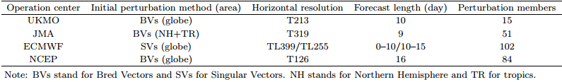
The forecast data of each model cover the periodof 1 June to 31 August 2007, with the forecast area inthe Northern Hemisphere(10°–87.5°N, 0°–360°), thehorizontal resolution of 2.5°×2.5°, and the forecastlead time of 24–168 h. The NCEP/NCAR reanalysisdata for the corresponding meteorological variableswere used as “observed values”. Note the area and the horizontal resolution of the NCEP/NCAR reanalysisdata are consistent with those of the TIGGEdata.2.2 Methodology2.2.1 Linear regression based superensemble forecasting
The multimodel superensemble forecast is formulatedafter Krishnamurti et al.(2000a, 2003). Ata given grid point, for a certain forecast time and meteorological element, the superensemble forecastingmodel can be constructed as:
where St represents the real-time superensemble forecastvalue, O the mean observed value during thetraining period, Fi, t the ith model forecast value, Fithe mean of the ith model forecast value in the trainingperiod, ai the weight of the ith model, n the numberof models participating in the superensemble, and t istime.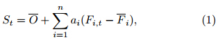
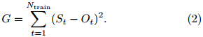
The weight ai can be calculated by minimizingthe function G in Eq.(2)below with the least squaremethod. The acquired regression coefficient ai willbe implemented in Eq.(1), which creates the superensembleforecasts in the forecasting period.
It should be noted that the traditional superensembleemploys a fixed training period of a certainlength, while an improved superensemble proposedby Zhi et al.(2009a)applies a running trainingperiod, which chooses the latest data of a certainlength for the training period right before the forecastday. The linear regression based superensemble usingrunning training period will be abbreviated as LRSUPhereafter.2.2.2 Nonlinear neural network based superensemble forecasting
In addition to the linear regression method, thethree-layer back propagation(BP)of nonlinear neuralnetwork technique(Geman et al., 1992; Warner and Misra, 1996)is implemented for the superensembleforecast(hereafter abbreviated as NNSUP). Duringthe training period, the output from each model istaken as the input for the neural network learning matrix.During the forecast period, the well-trained networkparameters are carried into the forecast model toobtain the multimodel superensemble forecasting(Stefanova and Krishnamurti, 2002; Zhi et al., 2009b).2.2.3 Bias-removed ensemble mean and multimodel ensemble mean
Bias-removed ensemble mean(hereafter abbreviatedas BREM)is defined as
where BREM is the bias-removed ensemble mean forecastvalue, and N the number of models participatingin the BREM. The running training period is alsoadopted in the BREM technique.
In addition, the multimodel ensemble mean(hereafterabbreviated as EMN)is performed and used asa cross-reference for the superensemble forecasts.

In the verification of the single model forecasts and evaluation of the multimodel ensemble forecasts, the root-mean-square error(RMSE)is employed.
where Fi is the ith sample forecast value, and Oi isthe ith sample observed value.3. Results3.1 Comparative analyses of linear and nonlinear superensemble forecasts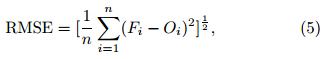
Based on the ensemble mean outputs of the 24–168-h ensemble forecasts of surface temperature inthe Northern Hemisphere from the ECMWF, JMA, NCEP, and UKMO, the multimodel superensembleforecasting was carried out for the period of 8–31 August2007(24 days). The length of the running trainingperiod was set to be 61 days.
As shown in Fig. 1, for the 24–168-h forecasts inthe entire forecast period, the superensemble forecasts(LRSUP and NNSUP)together with the multimodelEMN and BREM reduced the RMSEs by some meanscompared with the single model forecasts. With theextension of forecast lead time, the forecast skill improvementdecreased. For the 24–120-h forecasts, theRMSEs of the LRSUP and NNSUP were much smallerthan those of the single model forecasts, and theBREM also had improved forecast skills to some extent.When the forecast lead time was longer, e.g., 144–168 h, the BREM forecast skill caught up withthat of LRSUP and NNSUP in terms of the RMSEs.Therefore, for the summer Northern Hemisphere surfacetemperature, the multimodel ensemble forecastperformed better than the single model forecast. Althoughthe forecast improvement decreased with theforecast lead time, the forecast results remained stable.The NNSUP was skillful and outperformed theBREM and LRSUP for the 24–120-h forecasts. Butfor the 144–168-h forecasts, the errors of the BREM, LRSUP, and NNSUP were approximately equal.
 |
| Fig. 1. RMSEs of the surface temperature forecasts from the ECMWF, JMA, NCEP, and UKMO together withthe multimodel ensemble mean(EMN), bias-removed ensemble mean(BREM), linear regression based superensemble(LRSUP), and neural network based superensemble(NNSUP)at(a)24 h, (b)48 h, (c)72 h, (d)96 h, (e)120 h, (f)144h, and (g)168 h from 8 to 31 August 2007 in the Northern Hemisphere(10°–80°N, 0°–360°). |
In addition, the above analysis shows that theNNSUP was reasonably better than the other forecastschemes, because the NNSUP scheme might havereduced the forecast errors caused by the nonlineareffect among various models. However, repetitive adjustmentof the neural network parameters had to beperformed to obtain the optimal network structure, which slowed down the operation efficiency. Meanwhile, BREM and LRSUP had the advantage of beingcomputationally simple with reasonable accuracy;they were easier to be implemented for forecastersin their daily operation. In the following, the multimodelensemble forecast schemes of BREM and LRSUP(hereafter further abbreviated as SUP)will beemployed to give a multimodel consensus forecast of500-hPa geopotential height and temperature as wellas the zonal and meridional wind fields for comparativeanalysis.3.2 SUP and BREM forecasting of 500-hPa geopotential height
The SUP method for 24–72-h forecasts of the 500-hPa geopotential height had a high forecast skill. Especially, for 24-h forecast, it performed much betterthan the optimal single model forecasting(figure omitted).Figure 2a shows that the average RMSE of the96-h SUP forecasts was very close to that of the bestsingle model ECMWF forecast, while the BREM hada lower forecast skill than the ECMWF forecast mostof the time. For longer forecast lead time, this wasalso the case(figure omitted).
The overall low forecast skill of the SUP and BREM at longer than 96-h forecast lead time maybe attributed to the difference in the forecasting capabilityof each model in different latitudes as well asthe systematic errors of the models. In addition, itis unreasonable that the length of the training periodat all grid points is fixed at 61 days for the SUP and BREM. In the following, the optimal length of therunning training period will be examined at each gridpoint before the SUP and BREM forecasts are conducted.
As shown in Fig. 2, the RMSEs of the superensemblewith optimized training(O-SUP)are smallerto some extent than those of the superensemble withoutoptimized training(SUP). The optimal BREM(OBREM)forecast is also better than the BREM forecast.
 |
| Fig. 2. RMSEs of the 96-h forecasts of geopotential height at 500 hPa from the ECMWF by using(a)the superensemblewith(O-SUP) and without(SUP)optimized training and (b)the bias-removed ensemble mean with(O-BREM) and without(BREM)optimized training at each grid over the area 10°–60°N, 0°–360°. The ordinate denotes the RMSE and the abscissa denotes forecast date. |
To sum up, the 24–72-h forecast experiments of500-hPa geopotential height in the Northern Hemisphereshow that the improvement of SUP over theindividual models was more obvious, and the BREMforecast skill was somehow inferior to that of SUP.But for longer than 96-h forecast lead time, both SUP and BREM forecast schemes might not well reduce theoverall errors in the region. However, after the lengthof the running training period was optimized at eachgrid point, the forecast errors declined to some extent.
Zhi et al.(2009b)indicated that for the 24–168-hsuperensemble forecasts of the surface temperature inthe Northern Hemisphere, the optimal length of thetraining period is about two months. Since the forecastskill becomes lower when taking a longer trainingperiod in the BREM forecast, for shorter forecast leadtime of 24–72 h, the most appropriate training periodis about half month. For 96–168-h forecasts, it is suitableto select about one month as the optimal lengthof the training period. This shows that the selectionof the length of the training period is essential for theSUP and BREM forecasts. Only when appropriatelength is selected, can the forecast error be reduced toa minimum. Too long or too short training periodsmay influence the forecast skill. For forecasts at differentlead time, SUP and BREM forecasts also needdifferent optimal training periods.
In order to obtain the best forecast skill, the optimallength of the training period should be determinedfor the SUP forecast. As the models involved in themultimodel ensembles contribute differently for differentforecast regions, the length of the training periodfor each grid point should be tuned. As shown in Fig. 3, for most areas in the Northern Hemisphere, theoptimal length of the BREM training period is lessthan that of the SUP training period. Generallyspeaking, for both of the BREM and SUP schemes, thelength of the training period changes significantly fromone area to the other, which may be caused by differentforecasting system errors associated with eachmodel involved in the ensemble in different geographicalregions. At present, due to lack of data, it isdifficult to analyze the features of the changes in theoptimal length of the training period for different seasonswithin each region.
 |
| Fig. 3. Distributions of the optimal length(days)of the running training period for the 144-h forecasts of 500-hPageopotential height using the(a)BREM and (b)SUP techniques over the Northern Hemisphere. |
Figure 4 shows the forecast RMSEs of the 500-hPageopotential height, zonal wind, meridional wind, and temperature of the best single model, the EMN, theoptimal BREM, and the optimal SUP averaged in theforecast period in the Northern Hemisphere excludinghigh latitudes(10°–60°N, 0°–360°). As shown in Fig. 4a, the RMSEs of the 24–168-h best single model forecastsof the 500-hPa geopotential height range from10.4 to 37.7 gpm. The RMSE of SUP has always beenthe lowest for 24–120-h forecasts. Overall, the averageerror of the 24–120-h SUP forecasts is about 15 gpm, which reduces the RMSE by 16% compared with thebest single model forecasts. For 24–120-h forecasts, the BREM forecast has a lower skill than the SUPforecast.
 |
| Fig. 4. RMSEs of(a)500-hPa geopotential height, (b)zonal wind, (c)meridional wind, and (d)temperature forecastsfor the best individual model, the EMN, the optimal BREM, as well as the optimal SUP averaged for the forecast period17–31 August 2007 in the area 10°–60°N, 0°–360°. |
However, when the forecast lead time is extendedto 144–168 h, BREM has an approximately equal forecastskill as SUP. As shown in Figs. 4b–4d, similarconclusions are found for other variables at 500 hPa.For 144–168-h forecasts of 500-hPa temperature, theRMSEs of the SUP and BREM forecasts can still bereduced respectively by 8% and 10% compared withthe best single model forecasts(Fig. 4d).
Figure 4 shows that SUP can effectively improvethe forecast skill of all the studied variables at 500hPa. For the 24–120-h forecasts, SUP is superior toBREM, EMN, as well as the best single model forecast.Especially, the 24–120-h forecast error of the 500-hPageopotential height from SUP is 16% less than that ofthe best single model forecast, while that of BREM erroris about 8%. For the 144–168-h forecasts, the SUP and BREM forecast skills are approximately equal.3.4 Effect of the model quality on SUP and BREM
Krishnamurti et al.(2003)indicated that the bestmodel involved in the superensemble contributes toapproximately 1%–2% improvement for the superensembleforecast of the 500-hPa geopotentialheight, while the overall improvement of the superensembleover the best model is about 10%. Thisimprovement in the superensemble is a result of theselective weighting of the available models during thetraining period. That is to say, the weight distributionof all the models contributes a lot to the improvementof the superensemble forecasting techniques. Thenhow will a poor model affect the SUP and BREM?From a detailed analysis of forecast errors in Fig. 1, we have found that the UKMO model has the largesterrors among the four models participating in the ensemble.Now, two kinds of forecast schemes are designedto investigate the effect of model quality on themultimodel ensemble forecasting.
Scheme I: multimodel forecast including theUKMO forecast data.
Scheme II: removing the UKMO forecast datafrom the multimodel ensemble.
The training period and the forecast period arethe same as the above for the two schemes. Figure 5 gives the RMSEs of the SUP and BREM using theoriginal results of the multimodel data(4-SUP and 4-BREM), as well as SUP and BREM after removal ofthe UKMO data(3-SUP and 3-BREM).
 |
| Fig. 5. RMSEs of(a)geopotential height, (b)zonal wind, (c)meridional wind, and (d)temperature at 500 hPa fromthe optimal 4-SUP and 4-BREM and the optimal 3-SUP and 3-BREM with the worst model data excluded from themultimodel suite. The results were averaged for the period 17–31 August 2007 over the area 10°–60°N, 0°–360°for24–168-h forecasts. |
As shown in Fig. 5, the 3-BREM(without theUKMO model)forecast error is less than that of the 4-BREM(with UKMO). Take 24- and 168-h forecasts of500-hPa geopotential height as examples, RMSEs havebeen reduced from 10.4 and 37.7 gpm to 7.8 and 34.6gpm, respectively. The results show that the BREMforecast is sensitive to the performance of each modelinvolved in the ensemble. The better the model involvedis, the higher skill the multimodel ensembleforecast will have. Therefore, it is necessary to examinethe performance of each model involved beforeconducting the BREM forecast.
However, as shown in Fig. 5, the skill of the 24–168-h SUP forecast of each variable differs from thatof the BREM forecast. The forecast errors of 3-SUPwithout the UKMO model and 4-SUP including theUKMO model are approximately equal, i.e., the SUPforecast is not very sensitive to the poor model involved.The reason for this is that the SUP methoditself requires the models participating in the ensembleto have certain spread. For the UKMO model, although the forecast error of this model is large, it isstill within the spread. In addition, the poor modelwill be assigned a small weight in the SUP forecast.Thus, the inferior model has a small impact on theSUP results.3.5 Geographical distribution of the improvement by SUP and BREM over the best model
A detailed examination in Fig. 6 shows that the144-h forecast skills of the 500-hPa geopotential height and temperature are improved significantly by usingthe SUP and BREM forecast techniques in most areas, especially in the tropics. In the extratropics, theSUP and BREM forecast skills have been improvedby more than 20% in the areas of Ural Mountains, Lake Baikal, and the Sea of Okhotsk compared withthat of the best single model forecast. It is well knownthat Eurasian blockings frequently occur over the UralMountains, Lake Baikal, and the Sea of Okhotsk(Zhi and Shi, 2006; Shi and Zhi, 2007), which has a significantimpact on the persistent anomalous weathersin the upstream and downstream regions. The aboveanalysis indicates that the multimodel ensemble forecastsmay significantly improve the forecast skills ofthe variables at 500 hPa in mid–high-latitudes. Therefore, it is helpful for improving the forecast of somehigh-impact mid-high latitude weather systems by usingthe multimodel ensemble forecast techniques.
 |
| Fig. 6. Geographical distributions of the reduction percentage(%)of the mean RMSEs of 500-hPa geopotential height(left panels) and temperature(right panels)over the best model by the EMN(top panels), the optimal BREM(middlepanels), and the optimal SUP(bottom panels)for 144-h forecasts from 17 to 31 August 2007 in the Northern Hemisphere(10°–87.5°N, 0°–360°). |
The superensemble forecasting takes full advantageof multimodel forecast products to improve theforecast skill. Through series of comparative analysis, the following conclusions are obtained.
(1)Comparative analysis of linear and nonlinearmultimodel ensemble forecasts shows that for 24–120-h forecasts, the NNSUP forecast performs better thanLRSUP and BREM forecasts. However, for 144–168-hforecasts, the forecast errors of BREM, LRSUP, and NNSUP are approximately equal.
(2)Both LRSUP(or SUP) and BREM forecastsof 500-hPa geopotential height have different optimallengths of training period at each grid point. Theoptimal length of the training period for SUP is morethan one and a half months in most areas, while it isless than one month for BREM.
(3)The SUP forecasts using the optimal length ofthe training period at each grid point have roughly a16% improvement in the RMSEs of the 24–120-h forecastsof 500-hPa geopotential height, temperature, zonal wind, and meridional wind, while the improvementof the BREM is only 8%. But for 144–168-hforecasts, the forecast skill of the SUP is comparableto that of the BREM.
(4)For 24–168-h forecasts of the 500-hPa geopotentialheight, temperature, and winds, the BREMforecast without the UKMO model is more skillfulthan that with the UKMO model, while the SUPforecast error without the UKMO model is equivalentto that with the UKMO model. Hence, it is necessaryto verify each model involved before conducting theBREM forecasting.
Acknowledgments. We are grateful to Drs.Zhang Ling and Chen Wen for their valuablesuggestions.
| [1] | Bougeault, P., and Coauthors, 2010: The THORPEX Interactive Grand Global Ensemble. Bull. Amer. Meteor. Soc., 91, 1059–1072, doi: 10.1175/2010BAMS2853.1. |
| [2] | Buizza, R., D. Richardson, and T. N. Palmer, 2003: Benefits of increased resolution in the ECMWF ensemble system and comparison with poor-mans ensembles. Quart. J. Roy. Meteor. Soc., 129, 1269–1288. |
| [3] | Cartwright, T. J., and T. N. Krishnamurti, 2007: Warm season mesoscale super-ensemble precipitation forecasts in the southeastern United States. Wea. Forecasting, 22, 873–886. |
| [4] | Geman, S., E. Bienenstock, and R. Doursat, 1992: Neural networks and the bias/variance dilemma. Neural Computation, 4, 1–58. |
| [5] | Krishnamurti, T. N., C. M. Kishtawal, T. LaRow, et al., 1999: Improved weather and seasonal climate forecasts from multimodel superensemble. Science, 285, 1548–1550. |
| [6] | —–, —–, Z. Zhang, et al., 2000a: Multimodel ensemble forecasts for weather and seasonal climate. J. Climate, 13, 4197–4216. |
| [7] | —–, —–, D. W. Shin, et al., 2000b: Improving tropical precipitation forecasts from multianalysis superensemble. J. Climate, 13, 4217–4227. |
| [8] | —–, K. Rajendran, and T. S. V. Vijaya Kumar, 2003: Improved skill for the anomaly correlation of geopotential height at 500 hPa. Mon. Wea. Rev., 131, 1082–1102. |
| [9] | —–, C. Gnanaseelan, and A. Chakraborty, 2007a: Forecast of the diurnal change using a multimodel superensemble. Part I: Precipitation. Mon. Wea. Rev., 135, 3613–3632. |
| [10] | —–, S. Basu, J. Sanjay, et al., 2007b: Evaluation of several different planetary boundary layer schemes within a single model, a unified model and a multimodel superensemble. Tellus A, 60, 42–61. |
| [11] | —–, A. D. Sagadevan, A. Chakraborty, et al., 2009a: Improving multimodel forecast of monsoon rain over China using the FSU superensemble. Adv. Atmos. Sci., 26(5), 819–839. |
| [12] | —–, A. K. Mishra, and A. Chakraborty, 2009b: Improving global model precipitation forecasts over India using downscaling and the FSU superensemble. Part I: 1–5-day forecasts. Mon. Wea. Rev., 137, 2713–2734. |
| [13] | Leith, C. E., 1974: Theoretical skill of Monte Carlo forecasts. Mon. Wea. Rev., 102, 409–418. |
| [14] | Lorenz, E. N., 1969: A study of the predictability of 28-variable atmosphere model. Tellus, 21, 739–759. |
| [15] | Mishra, A. K., and T. N. Krishnamurti, 2007: Current status of multimodel super-ensemble and operational NWP forecast of the Indian summer monsoon. J. Earth Syst. Sci., 116, 369–384. |
| [16] | Park, Y.-Y., R. Buizza, and M. Leutbecher, 2008: TIGGE: preliminary results on comparing and combining ensembles. Quart. J. Roy. Meteor. Soc., 134, 2029–2050. |
| [17] | Rixen, M., and E. Ferreira-Coelho, 2006: Operational surface drift forecast using linear and nonlinear hyper-ensemble statistics on atmospheric and ocean models. J. Mar. Syst., 65, 105–121. |
| [18] | —–, J. C. Le Gac, J. P. Hermand, et al., 2009: Superensemble forecasts and resulting acoustic sensitivities in shallow waters. J. Mar. Syst., 78, S290–S305. |
| [19] | Shi Xiangjun and Zhi Xiefei, 2007: Statistical characteristics of blockings in Eurasia from 1950 to 2004. Journal of Nanjing Institute of Meteorology, 30(3), 338–344. (in Chinese) |
| [20] | Stefanova, L., and T. N. Krishnamurti, 2002: Interpretation of seasonal climate forecast using brier skill score, FSU superensemble, and the AMIP-I data set. J. Climate, 15, 537–544. |
| [21] | Toth, Z., and E. Kalnay, 1993: Ensemble forecasting at NMC: The generation of perturbations. Bull. Amer. Meteor. Soc., 74, 2317–2330. |
| [22] | Warner, B., and M. Misra, 1996: Understanding neural networks as statistical tools. J. Amer. Stat., 50, 284–293. |
| [23] | Zhi Xiefei and Shi Xiangjun, 2006: Interannual variation of blockings in Eurasia and its relation to the flood disaster in the Yangtze River valley during boreal summer. Proceedings of the 10th WMO International Symposium on Meteorological Education and Training, 21–26 September 2006, Nanjing, China. |
| [24] | Zhi Xiefei, Lin Chunze, Bai Yongqing, et al., 2009a: Superensemble forecasts of the surface temperature in Northern Hemisphere middle latitudes. Scientia Meteorologica Sinica, 29(5), 569–574. (in Chinese) |
| [25] | —–, —–, —–, et al., 2009b: Multimodel superensemble forecasts of surface temperature using TIGGE datasets. Preprints of the Third THORPEX International Science Symposium, 14–18 September 2009, Monterey, USA. |
| [26] | —–, Wu Qing, Bai Yongqing, et al., 2010: The multimodel superensemble prediction of the surface temperature using the IPCC AR4 scenario runs. Scientia Meteorologica Sinica, 30(5), 708–714. (in Chinese) |