Forests are affected by various disturbance factors (e.g., fire, disease and insect infestation, and logging) and non-disturbance factors(e.g., temperature, wetness, and precipitation). Disturbance factors are closely associated with carbon stock and can be interpreted to obtain forest vertical structure parameters and aboveground biomass (AGB). Li et al. (2011) utilized a vegetation change tracker(VCT) algorithm to extract disturbance information from Landsat time series data and applied a regression tree model to estimate forest tree height in the Mississippi region (R²=0.91, RMSE=1.97 m). Pflugmacher et al. (2012)demonstrated that although Lidar parameters could predict forest AGB_live most accurately (R²=0.88), AGB_live (R²=0.80)predicted using time-series disturbance information was more accurate, than that based onsingle-scene Landsat data (R²=0.58). Using forest disturbance information showsa potential for estimating forest structural variables and biomass.

In NASA's land satellite (Landsat) program, eight satellites have been launched since July 23, 1972. Through more than 40 years of earth observation, a large body of data has been accumulated. Its high-resolution, longtime-series information provides a unique resource for recording forest disturbance and recovery history over the past few decades (Pflugmacher et al., 2014). The conventional method of acquiring disturbance information based on Landsat images is to only compare two images of one surface feature (Cohen et al., 2002; Olsson, 2009). However, this method can neitheradequately reveal the interrelationships among multi-temporal imagesnor separate background noise from subtle vegetation change. To exploit longtime-series satellite data and increase the signal-to-noise ratio during detection of spectral changes, researchers have been attempted to use multi-period images to run joint analyses to identify forest disturbance and recovery information (Healey et al., 2006; Goodwin et al., 2008). Since the U.S. Geological Survey(USGS) began to offer a free downloading service for longtime-series Landsat data, multi-period image joint analysis methods have been began to develop rapidly (Garcia-Haro et al., 2001; Huang et al., 2010; Hostert et al., 2003; Vogelmann et al., 2011). Kennedy et al. (2010a) proposed that Landsat-based detection of trends in disturbance and recovery(LandTrendr) can be used to identify different types of disturbance events and can provide post-disturbance forest recovery information.

In disturbance-monitoring studies, multi-spectral bands are usually converted to indices characterizing forest growth conditions for quantitative analysis(Tab. 1). Constructing disturbance-monitoring indices is the basis for identification of the disturbance signal and can enhance the spectral response of forest change. Generally, indices constructed based on IR and near-IR shortwave bands have better capabilities of identifying forest disturbance than indices constructed on the basis of visible band (Schroeder et al., 2011; Main-Knorn et al., 2013).

In this study, we identified forest disturbance information based on Landsat thematic mapper and enhanced thematic mapper plus (TM and ETM+) time-series data by means of the LandTrendr method using two disturbance-monitoring indices, the tasseled-cap angle(TCA) and the tasseled-cap distance(TCD). The TCA index wasproposed based on greenness and brightness components, for describing variation of forest vegetation coverage by constructing the included angle of both components in the vegetation plane(Powell et al., 2008). The TCD index was proposed by Duane et al.(2010) and denotingthe distance between brightness and greenness components in the vegetation plane; it is used to describe forest structure and composition. Both indices are used to study forest parameters, being capable of effectively enhancing the spectral response of forest change (Pflugmacher et al., 2012; 2014; Duane et al., 2010).

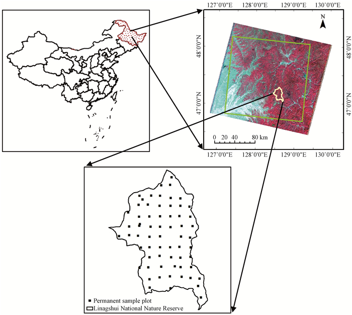
1 Research area and methodology 1.1 Research area

The study area is located at the centerof the Lesser Xingan Moutains, covering Dailing and Liangshui tree farms (Fig. 1). Its forest type is dominantly of mixed conifer-broadleaf forest. The study area is covered by a single-scene Landsat image.

1.2 Data source 1.2.1 Remote sensing imagery data

A total of 33 periods of Landsat TM and ETM+ images with path/row numbers of 117/27 during 1984—2006 were used to calculate forest disturbance and recovery parameters (Tab. 2). All images were Landsat CDR reflectance data pre-processed by the Landsat ecosystem disturbance adaptive processing system (LEDAPS) and downloaded from http://earthexplorer.usgs.gov/. Data acquisition times are centered on the forest growth period (July-August) with every year corresponding to two scenes of imagery on average, providing adequate data for computation of disturbance parameters.

1.2.2 Forest resource survey data

The forest survey data of the study area consist of forest resource data from successive checks of fixed plots(standard plots) in 2005 and complementary plot data from field surveys. The subcompartment data were divided into subregions of different areas based on forest conditions and operation level. Each subregion exhibitsthe same stand structure features; information such as stand type, yield class, forest canopy density, and stand volume, were mainly documented. Fixed plots were laid out on a kilometer grid of intersecting points on a terrain map with a scale of 1:50 000. The plot spacing was 1 km × 1 km, with the area of every fixed plot being 0.06 hm². Measurement factors included mean tree height, mean diameter at breast height(DBH), forest age, tree species structure, and total vegetation coverage. Surface survey data were square plots with a side length of 30 m × 30 m. Tally information was documented and plot centercoordinates were positioned using the Differential Global Positioning System (DGPS). The diameter of each tree at a height of 1.3 m above the rhizome(DBH) was measured with diameter tape; canopy diameters in four directions (east, west, south, and north) were measured with a tape measure; and the height of each tree was measured with a laser rangefinder (TruPulse 360). For the study area, DBH ranged from 4.4 to 58.7 cm and tree height ranged from 1.8 to 32.6 m(Tab. 3).

1.3 Methodology 1.3.1 Calculation of disturbance parameters

LandTrendr is a method of extracting ground spectral change trajectories from yearly time-series data. It is capable of capturing short-term changes of a time series and smoothing long-term trends.The original series of spectral response changes was segmented and linearly fitted using a time-series segmentation algorithm, so the data were transformed into a series of line segments. Perchance in line segment trend, time-series features including disturbance year and forest recovery were captured. The process flow of extracting forest disturbance and recovery information with LandTrendr from multiple time-series Landsat data can be described as complicating followed by simplifying; that is, one builds a maximally complex time trajectory fitting the model first, then iteratively processes the fitting result to simplify the model and eliminate the noise spike signal. The algorithm consists of six steps:

1) Extracting the spectral time series. For time series images, several pre-processes, such as geometric correction, atmospheric correction, and radiometric correction, were run. Disturbance-monitoring indices were calculated, spectral information was extracted from every disturbance-monitoring index image by using a moving window averaging method, and a time-series profile of each pixel was obtained.

2) Removing noise. Although clouds and shadows were masked out at the time of image pre-processing, residual noise would remain in the image; in the LandTrendr method, noise-induced change in the time-series profile is assumed transient and that pre-spike and post-spike values are basically constant. Conversely, a profile change induced by a disturbance or recovery is more persistent, and profile values before and after the occurrence of a disturbance or recovery event would differ obviously. Therefore, according to the similarity threshold (despike) in the control file, the LandTrendr algorithm iteratively deletes spikes having a noise characteristic in the profile. The worst peak was deleted at each iteration until the threshold requirement was satisfying.

3) Identifying potential vertices. A vertex on a time-series trajectory (corresponding to a spectral value for the year when disturbance change occurs) joins different time intervals. LandTrendr uses residual-error-based time-series segmentation to identify vertices, runs a least-square regression computation to get a fitting result with spectral values corresponding to start and end years on the trajectory as initial vertices, and then predicts the spectral value for every year according to the fitting result and sets the year with the maximum absolute difference between the true value and the predicted value as a new vertex. The new node will segment the time-series trajectory into two portions and run a regression of both portions and calculate mean square errors (MSEs). For the portion of the trajectory with the larger MSE, the above operation was repeated to seek a new vertex. The iterative regression operation was run repeatedly until the acquired vertex count and the segment count satisfy the corresponding settings in the control file (max_segments + vertex count overshoot). To prevent over fitting, one must judge the convergence of the segmentation result according to an angle criterion, calculate the angles among segments, and iteratively cull the vertex and line segment with the shallowest angle until the threshold (max_segments) setting is met.

4) Fitting trajectories. After vertices were identified, regression-based and point-to-point-based connection approaches were used to fit the time series. Starting from the first vertex, fitting results of both approaches were compared, and the approach with the smaller MSE was used to fit the line segment. Because the start point of the second line segment is the end point of the first line segment, both approaches were used to compute the MSE, then the computed results of the regression connection and the point-to-point connection approaches were compared to select the better fit. All vertices were computed in order and finally, a set of successively connected line segments were obtained in place of the original time-series trajectories. The P value for the F-statistic of the fitting results was then calculated. If it satisfied the threshold (pval) specified in the control file, then the next operation was run; otherwise, the trajectory was refitted.

5) Simplifying model. Based on the complex model, previous, iterative computations proceeded according to the recovery threshold in the control file or MES rule. For each iterative computation, the weakest vertex was removed and the remaining vortexes were refitted until the number of segments is 1.

6) Determining the best model. During model simplification, once a vertex was deleted, the trajectory would be refit to generate a P value for the F-statistic. These P values were compared and the optimal model was selected to get the final time-series reconstruction result.

Time series data processing with the LandTrendr algorithm relate to use of multiple parameters in the control file (Tab. 4). Kennedy et al.(2010a) used the Timesync tool to evaluate in detail the parameters in the LandTrendr control file and determine the optimal solution of each parameter, providing a reference for LandTrendr application research.

1.3.2 Model for forest canopy height

To evaluate the capability of disturbance parameters estimating forest structural variables, we built a forest parameter algorithm model with two groups of predictor variables (Tab. 5). One group of predictor variables included single-temporal spectral information without disturbance and recovery information. The other group of predictor variables comprised single-temporal spectral information with disturbance and recovery information added.

1.3.3 Accuracy evaluation

In this study, the root mean square error (RMSE) and the prediction accuracy (P) of the tree height of the measured plots and the tree height estimated by the model wereused to evaluate the quality and credibility of the model. RMSE is calculated as shown in Equation (1); the smaller the RMSE value between the tree height of the measured plots and the tree height estimated by the model is, the better the model estimates. P is calculated as shown in Equation (2); the closer the P value is to 1, the better the model prediction is.

$ {\rm{RMSE}} = \sqrt {\frac{1}{n}\sum\limits_{i = 1}^n {{{({y_i} - {{\hat y}_i})}^2}} } . $

(1)

In the formula, RMSE is the root mean square error, y_i is the measured tree height at the ith plot, $ {{{\hat y}_i}} $ is the tree height estimated by the model at the i th plot, and n is the number of plots.

$ P = (1 - \frac{{{t_{0.05}}{S_{\bar y}}}}{{}}) \times 100\% ; $

(2)

$ {S_{\bar y}} = \sqrt {\frac{{\sum {{{\left( {{y_i} - {{\hat y}_i}} \right)}^2}} }}{{n\left( {n - p} \right)}}} . $

(3)

In the formula, P is the prediction estimation, y_i is the measured tree height at the ith plot, $ {{{\hat y}_i}} $ is the tree height estimated by the model at the ith plot, p is number of parameters in model, n is thenumber of plots.

2 Results and analysis

The models for the relationship between the forest height and predictor variables (Tab. 5) were established using the Random Forests (RF) algorithm. The optimal model parameter combination of each RF model was found through a traversal analysis, and based on the out-of-bag mean square error MSE_OOB of the training set, an inversion model was determined. Tab. 6 shows the fitting result of the tree height RF model, which indicates that having more disturbance information, can increase the forest heightfitting accuracy.

2.1 Disturbance parameters

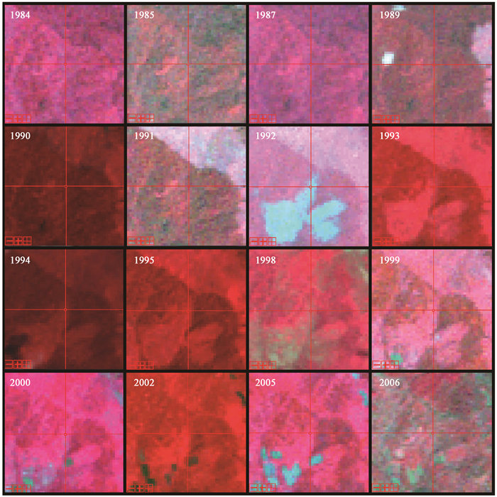
A down-trending line segment represents being disturbed, an up-trending line segment represents the post-disturbance recovery stage, and a horizontal line represents not being disturbed. As shown in Fig. 2, the forest was obviously disturbed in 1992 and its corresponding trajectory exhibited a downtrend; after 1992, the forest region no longer suffered disturbance and its corresponding fitting trajectory ramped up to the horizontal state. To quantitatively describe the trajectory, we extracted a series of disturbance data (Tab. 7) from the fitting profile. DBYEA and DBVAL correspond to year and spectral value, respectively, of point A in Fig. 3, DDUR corresponds to the time difference between points A and B; DMAG corresponds to value a, RBYEAR and RBVAL correspond to year and spectral value of point B, RMAG corresponds to value b, and RDUR corresponds to the time difference between points A and C.

Multiple disturbance recovery events might occur in a time series of one pixel, and we computed the maximal disturbance information of forest-land-type pixels only. B computation, four types of time series fitting trajectories can be obtained: disturbance followed by recovery, disturbance followed by non-recovery, recovery only, and no disturbance. For all types of trajectories, parameters were set according to the following rules:

1) If the time series of a pixel contains recovery information only, then DBYEA is set as the start year of the time series, DBVAL is set as the spectral value to which the start year corresponds, and DDUR and DMAG are defined as 0.

2) If the time series of a pixel contains disturbance information only, then RBYEAR is set as the end year of the time series, RBVAL is set as the spectral value to which the end year corresponds, and RMAG and RDUR are defined as 0.

3) If the time series of a pixel does not contain disturbance and recovery information, then all parameters are set as 0.

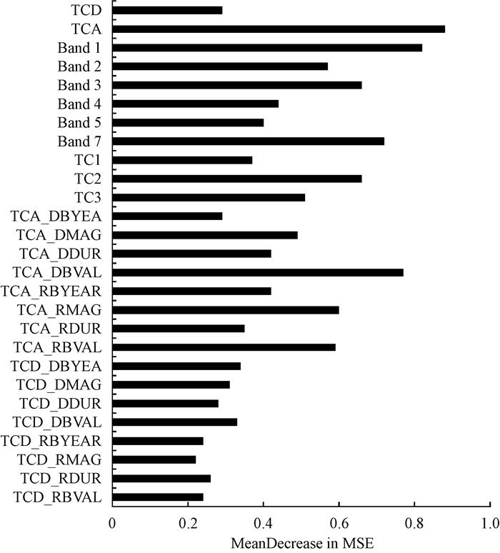
2.2 Importance of model variables

Variable TCA was the most important in the tree height inversion model (Fig. 4). The importance of disturbance parameters (spectral value prior to disturbance onset, spectral value for recovery start, and recovery magnitude) calculated on the basis of the TCA monitoring index were higher than those of TCD disturbance parameters, indicating that TCA disturbance parameters can more easily be interpreted to obtain tree height than TCD disturbance parameters.

2.3 Influences of disturbance parameters on model accuracy

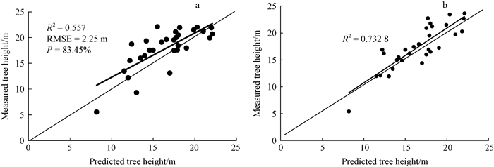
The RF inversion model was used to estimate tree height in the study area. Measured plot data were applied to validate the predicted result. Fig. 5 shows the result of validating tree height with plot data, from which increasing disturbance information enhances the correlation between spectral reflectance and the forest parameter and improves the prediction accuracy of the forest tree height model, with tree heightPrising from 83.45% to 89.79%.

3 Conclusion

The reconstructed time-series trajectories based on Landsatwere analyzed and 8 parameters describing forest disturbance features were extracted. Introducing disturbance parameters into forest height estimation modelscould improve the prediction accuracy of forest tree height from 83.45% to 89.79%, and enhance the correlation between spectral reflectance and the forest parameter tree height. Thus, use of forest disturbance information has positive potential for estimating forest structure parameters and biomass.

Conventional optical remote sensing data can becombinatorially transformed with IR and near-IR band reflectance to express forest parameter information.However, when vegetation coverage reaches a certain threshold, the spectral signal saturates and forest parameter estimation accuracy declines. In advanced, forest disturbance and recovery information obtained based ontime-series trajectory trend analysis is not subject to signal saturation, which could enhance the correlation between reflectance and forest parameters. Nevertheless, there is stilla challengeto validate disturbance parameters accurately due to the lack of historic data of forest disturbance.To solve this problem, we could tomake visual and manual interpretation based on high-resolution images (e.g., Google Earth).