 2016, Vol. 52
文章信息
- 崔令军, 张雄清, 段爱国, 张建国
- Cui Lingjun, Zhang Xiongqing, Duan Aiguo, Zhang Jianguo
- 基于分层贝叶斯法的杉木人工林最大密度线
- A Hierarchical Bayesian Model to Predict Maximum-Size Density Line for Chinese Fir Plantation in Southern China
- 林业科学, 2016, 52(9): 95-102
- Scientia Silvae Sinicae, 2016, 52(9): 95-102.
- DOI: 10.11707/j.1001-7488.20160911
-
文章历史
- 收稿日期:2015-04-23
- 修回日期:2016-06-02
-
作者相关文章


2. 南京林业大学南方现代林业协同创新中心 南京 210037
2. Collaborative Innovation Center of Sustainable Forestry in Southern China, Nanjing Forestry University Nanjing 210037
在植物生长过程中,随着植株的生长,越来越多空间被占据,导致可用的资源不足,最终引起一部分个体死亡,即自然稀疏(Westoby,1984; Hynynen,1993)。在林业上,自然稀疏法则常被用来构造相对密度指数(Drew et al.,1979)、密度控制图(Newton,2012)等,因此,分析自然稀疏规律对于林业管理者在实践上有很大的指导意义。
对于自然稀疏法则,讨论较多的是Reineke(1933)方程和Yoda等(1963)3/2法则。2位学者认为,对于一定的植物大小,必定存在一个最大的密度,即在一个林分生长演替过程中,存在着一条最大密度线。Reineke(1933)通过密度与平均直径的关系研究,发现最大密度线存在着固定斜率-1.605,而Yoda等(1963)研究发现,在自稀疏过程中,植物平均质量与密度之间的关系存在着固定斜率-1.5,即著名的3/2法则。之后,有研究者利用实地数据证明了Reineke和Yoda的结论: 最大密度线的斜率不随树种、林龄和立地质量的变化而变化,或者变化较小(Gadow,1986; Pretzsch et al.,2005)。然而,也有研究者对该结论提出了质疑,认为最大密度线的斜率是变化的(Bi et al.,1997;Pretzsch,2006)。Weiskittel等(2009)认为,最大密度线斜率估计方法不同是导致存在争议的主要原因之一。
估计最大密度线的方法主要有: 1)人为根据数据点波动范围的上限手绘最大密度线,并计算出斜率(Yoda et al.,1963; Drew et al.,1977);2)最小二乘法(Wilson et al.,1988; Yang et al.,2002),该方法简单,用得也比较多; 3)分位数回归法(Cade et al.,1999);4)主成分分析和压轴回归分析法(reduced major axis regression)(Wilson et al.,1999;Bégin et al.,2001);5)平分线回归法(bisector regression approach)(Newton,2006); 6)随机边界法(Bi,2001;2004)等。Zhang等(2005)对几种估计最大密度线的方法做了比较,发现随机边界法要优于最小二乘法、分位数回归法和主成分分析法。
在分析最大密度线时,取样往往来自不同的立地、经营措施(初始密度)等。而如果采用以上几种方法对这些数据进行分析,一般都先假设最大密度线的截距和斜率在不同立地条件或经营措施下一致; 但是此假设存在着一定的争议。混合效应模型分析方法能够很好地解决这个问题,即将立地环境或经营措施当作随机效应。VanderSchaaf等(2007)利用混合效应模型估计火炬松(Pinus taeda)最大密度线,发现混合效应模型要优于其他方法; 但是混合效应模型仅给出参数的点估计值,并未能体现出参数估计值的不确定性(Li et al.,2012)。
分层贝叶斯模型法(hierarchical Bayesian method)是分析分层数据和评价参数不确定性的一个很好方法; 而且贝叶斯法综合利用了先验信息和样本信息,先验信息是在进行统计推断时不可缺少的一个因素,可以来自历史文献资料或者主观信念,这在林业研究工作中是很重要的(张雄清等,2014)。杉木(Cunninghamia lanceolata)是重要的用材树种,分布于我国南方大部分地区,在我国南方林区的林业可持续发展中占有重要地位。国内一些学者对杉木最大密度线也做了些研究。吴承祯等(2000)在前人研究植物种群自然稀疏法则的基础上,根据生长的密度理论和若干假设,提出描述杉木种群密度变化的理论模型; 陈水松等(2006)研究了20年生杉木间伐试验林自然稀疏的变化,并构建了密度控制管理图; Sun等(2011)利用几种不同估计方法分析了杉木自然稀疏线(材积-密度),并选择出了最优估计方法等。但是对于分层贝叶斯法在杉木最大密度线的研究未见报道。本文以福建杉木密度试验林为研究对象,利用分层贝叶斯法分析杉木最大密度线,以期为杉木自然稀疏规律研究提供一种新思路。
1 试验地概况及数据整理试验地位于福建省邵武市卫闽林场,武夷山北段中山山脉东南侧山区(117°43′E,27°05′N)。主要地貌为低山、高丘,海拔一般在250~700 m之间。该地区属于亚热带季风气候,气温温和湿润,年均温17.7℃,1月和7月的平均温度分别为6.8 ℃和28 ℃。年降雨量1 768 mm,年平均相对湿度为82%,地理条件比较适宜杉木生长,是杉木的中心产区。
该试验林使用1 年生苗木于1982 年造林,采用随机区组试验设计,5 个密度:A 密度(2 m × 3 m)、B 密度(2 m × 1.5 m)、C 密度(2 m × 1 m)、D 密度(1 m × 1.5 m)、E 密度(1 m × 1 m),每个密度3 次重复,共15 个样地,每个样地面积600 m2。1983—1988年间逐年调查,1988 年后隔年调查,直到2010年。样地内每株树进行编号,对样地内林木进行每木检尺。孙洪刚等(2010)研究认为,当样地内枯损株数未达到总株数的10%时,杉木林分未开始进行自然稀疏,因此在拟合最大密度线时将这些数据剔除。本研究也采用相同方法对数据进行筛选,最终A密度的3个样地和B密度的1个样地都被排除掉,剩下11个样地,组成样本量为76的数据集。杉木林分中各变量统计值见表 1。
|
|
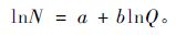
Reineke(1933)根据林分平方平均直径(Q)和每公顷株数(N)的关系,提出最大密度线方程:
|
(1) |
式中: a,b为待估参数; b为最大密度线的斜率。
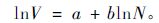
在Reineke(1933)方程中,认为b是一个常数,为-1.605。之后,Yoda等(1963)在此方程理论基础上,提出了植物平均生物量和密度的关系,并得到了著名的3/2法则。White(1981)认为树木的生物量和材积有着非常密切的关系,因此,在林业上一般将平均生物量用平均材积(V)代替,得到以下方程:
|
(2) |
在本研究中,利用Reineke(1933)方程分析杉木最大密度线,原因有以下3点: 1)Q是描述林分平均大小的常用变量之一,而且易获取; 2)Q与N和林分断面积关系很密切; 3)林木材积一般通过材积表查询得到。然而通过材积表获取的材积存在一定的误差,如果利用材积分析最大密度线[式(2)],那么就将此误差引进最大密度线方程中(Curtis et al.,2000),估计不准确。
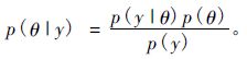
2.2 贝叶斯理论贝叶斯法是基于贝叶斯定理而发展起来的一种系统的统计推断方法。贝叶斯推断的基本原理是将待估参数的先验分布与样本信息结合,再根据贝叶斯定理得出后验分布信息,之后根据此后验分布信息去推断未知参数的分布(张雄清等,2014)。令y=(y1,y2,y3,…)为数据集,θ=(θ1,θ2,θ3,…)为待估的参数向量,则根据贝叶斯理论,其基本公式为:

|
(3) |
式中: p为概率分布函数或者密度函数。
在贝叶斯方法中,通过概率分布 p(θ|y) 描述参数θ的不确定性,进而估计参数θ。根据贝叶斯条件概率,θ的条件概率分布为:
|
(4) |
贝叶斯统计中,在给定样本数据y下参数θ的条件分布 p(θ|y) 即所需求参数的后验分布, p(y|θ) 是在给定θ下y的似然函数,p(θ)是θ的先验分布。
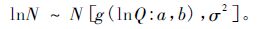
在本研究中,根据最大密度线方程(1),得到下式:
|
(5) |
式中: g(lnN:a,b)=a+blnN 。所以方程(3)可以写成:

|
(6) |
其中 p(样本|a,b) 为:
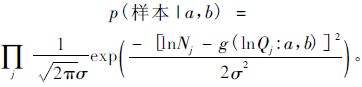
|
(7) |
初植密度对最大密度线是否有影响长期以来一直饱受争论。在本研究中,为分析初植密度对杉木最大密度线的影响,引入了分层贝叶斯模型。模型形式有3种: 1)在截距处考虑初植密度的随机效应,而斜率作为固定效应不变(M1); 2)在斜率处考虑初植密度的随机效应,而截距作为固定效应不变(M2); 3)同时在截距和斜率处考虑随机效应(M3)。3种方程形式如下:

|
(8) |

|
(9) |

|
(10) |
式中: u0i,u1i为随机效应参数,而且u0i~N(0,σ02),u1i~N(0,σ12),ε~N(0,σ2)。对于分层贝叶斯模型,模型的总方差有2个来源:组内波动性(within-group variability)和组间波动性(between-group variability),在本研究中,即不同初植密度间的波动性和相同初植密度内的波动性。
2.4 先验分布贝叶斯方法的一个重要特点是参数在抽样前就具有先验分布(Gelman et al.,2004)。在上述杉木最大密度线方程中,首先要为参数a,b构造合适的先验分布。有些学者提出利用无信息先验分布,对于无信息先验分布,一般选择均值为0、方差足够大的正态分布,使其能够覆盖整个数据范围的波动情况(Ellison,2004)。当然也可以选择有信息先验分布作为贝叶斯方法中的先验分布,这些先验信息可以来自文献资料或者主观信念。本研究中,对于斜率b,通过查阅相关文献,搜集树木自然稀疏的最大密度线的斜率值(表 2),构造先验信息分布。而对于截距a,则利用无信息先验分布。参数的先验信息分布见表 3。
|
|
|
|
对于模型的评价,一般采用决定系数(R2)和均方根误差(RMSE)作为模型的拟合统计量指标。均方根误差公式为:

|
(11) |
式中: yi 为实际值;$\bar{y}$i,yi 分别为预测值和平均值;n为观察个数。
在本研究中,同时还利用DIC统计量判断贝叶斯模型拟合的效果(Spiegelhalter et al.,2002)。与RMSE一样,DIC越小,说明模型拟合越好。
|
(12) |
式中: DBAR=Eθ{-2lg[p(y|θ)]}, 表示模型拟合数据的优劣; PD为模型中参数的有效个数, PD=DBAR+2lg[p(y|θ-)], 表示模型的复杂度。
对于贝叶斯参数估计,利用WinBUGS软件(Spiegelhalter et al.,2003)。在该软件中,通过Gibbs抽样(Chib et al.,1995),利用马尔科夫链蒙特卡洛方法完成估计。在本研究中通过R2WinBUGS(Sturtz et al.,2005)连接R软件和WinBUGS软件完成,同时输出图形。在估计参数时,为了保证迭代收敛和得到稳定的参数后验概率值,迭代次数设为10万次,并去掉前面的5 000次退火(burn-in)迭代。
4 结果与分析在杉木最大密度线方程中,分别利用普通贝叶斯模型和分层贝叶斯模型估计最大密度线的截距和斜率,得到估计值和模型评价指标,见表 4。虽然分层贝叶斯模型的R2比普通贝叶斯模型大,均方根误差RMSE比普通贝叶斯模型的小,但是参数估计值a和b与普通贝叶斯相近;而且,也发现普通贝叶斯的DIC绝对值小于M1模型、大于M2模型。综合DIC,R2和RMSE比较可发现,M2模型要比其他模型好。
|
|
基于模型M2,得到图 1。杉木最大密度线的截距和斜率服从一定的正态分布,这也很好地解释了最大密度线的截距和斜率不是固定不变的,而是存在着一定的不确定性。此外,根据模型M2,得到杉木最大密度线图,见图 2。通过分层贝叶斯估计所拟合的最大密度线相对较好,但是对于最大密度线的上界有一定的低估。

|
图 1 杉木最大密度线的截距和斜率的后验概率分布(M2) Fig.1 Posterior density curves of maximum-size density curve of Chinese fir for model M2 |

|
图 2 杉木最大密度线及95%区间(M2) Fig.2 Maximum-size density curve and 95% interval of Chinese fir for model M2 |
另外,通过表 4也发现,根据T-检验,随机效应方差( σ02,σ12 )不管是在截距上( σ02 =0.008,SD=0.029)还是斜率上( σ12 =0.003,SD=0.016),其t值都小于1.96,差异不显著,由此可推断初植密度对杉木最大密度线的斜率和截距都没影响。因此,在表 4中未列出M3的值。在模型M1中可发现,总方差为0.035,其中初植密度间的波动性所带来的方差为0.008; 换而言之,只有22.86%的方差是由于不同初植密度所造成的,而剩下77.14%的方差是由于相同初植密度内重复测量所造成的。这同样的问题在模型M2中也可发现,由初植密度所带来的方差仅占总方差的10%。
5 结论与讨论对于最大密度线争论较多的是斜率是否为常数。有些学者认为斜率是常数,不随树种、林龄、立地等因子的变化而变化(Puettmann et al.,1993; Tang et al.,1995; Yang et al.,2002); 然而,有些学者却认为最大密度线的斜率随着初植密度的不同而异(Turnblom et al.,2000; VanderSchaaf et al.,2007)。本研究发现,初植密度并没有对杉木最大密度线的斜率造成影响,且初植密度在截距上的随机效应不显著,因此也可理解为初植密度对杉木最大密度线的截距影响不显著,与其他一些研究(Weiskittel et al.,2009; Leon,2011)不同。由于初植密度的随机效应不论在截距上还是在斜率上都不显著,因此最大密度线模型的不确定性在很大程度上是由相同初植密度内不同样地的重复测量所造成的。Zeide(2001)发现林龄和环境的变化能够使得树木的自然稀疏发生变化。Harrington(1986)和Weiskittel等(2009)研究发现赤桦木(Alnus rubra)的最大密度线对坡面、土壤水分、干燥度等很敏感。因此,最大密度线在不同的样地存在一定的不确定性,这也可以从本文的图 1反映出来。
尽管对于最大密度线的估计已经有很多种方法,但是这些方法都存在一定的局限性。如通过手绘的方法画最大密度线比较主观、武断(Drew et al.,1977); 分位数回归(Scharf et al.,1998; Cade et al.,1999)估计最大密度线波动性比较大,甚至数据微小的变化都会使得估计结果产生较大的波动(Scharf et al.,1998; Cade et al.,2003); 最小二乘法描述的是数据的平均状态,这显然与实际的情况不符(孙洪刚等,2010)。Bi等(2000)利用随机边界法分析最大密度线,得到较理想的结果。然而这些方法忽略了最大密度线的波动性,而且也没有考虑重复测量间的相关性。在本研究中,提出利用分层贝叶斯模型分析杉木最大密度线,不仅能够很好地反映出杉木最大密度线的不确定性,而且也考虑了重复测量产生的相关性。另外,利用分层贝叶斯模型,引入最大密度线的斜率的先验信息分布,估计结果更加可靠,这也是贝叶斯方法估计的一大特点。本文所估计的杉木最大密度线的斜率的后验概率平均值为-1.882(M2),该值与WBE模型(West et al.,1997; 1999)计算所得的-2相近。而且,Mohler等(1978)研究10个树种纯林的最大密度线的斜率,得到这10个树种的斜率范围为-2.29~-1.750,本研究所得到的值属于这个范围。因此,利用分层贝叶斯模型分析杉木最大密度线能够为杉木最大密度线的研究提供一种新思路。当然,也可以在杉木人工林最大密度线方程中加入立地质量、环境变量等因素,使得先验分布更精确,进而提高杉木人工林最大密度线预测的可靠性。
| [1] |
陈水松, 陈长发, 何寿庆. 2006. 杉木林间伐强度自然稀疏与结构规律研究. 林业科学 , 42 (1) : 55–62.
( Chen S S, Chen C F, He S Q.2006. The natural thinning and structural pattern of the intermediate cutting intensity in the Cunninghamia lanceolata stand. Scientia Silvae Sinicae , 42 (1) : 55–62. [in Chinese] ) (  0) 0)
|
| [2] |
孙洪刚, 张建国, 段爱国. 2010. 数据点选择与参数估计方法对杉木人工林自疏边界线的影响. 植物生态学报 , 34 (4) : 409–417.
( Sun H G, Zhang J G, Duan A G.2010. A comparison of selecting data points and fitting coefficients methods for estimating self-thinning boundary line. Chinese Journal of Plant Ecology , 34 (4) : 409–417. [in Chinese] ) ( 0)
|
| [3] |
吴承祯, 洪伟. 2000. 杉木人工林自然稀疏规律研究. 林业科学 , 36 (4) : 97–101.
( Wu C Z, Hong W.2000. A study on the self-thinning law of Chinese fir plantation. Scientia Silvae Sinicae , 36 (4) : 97–101. [in Chinese] ) ( 0)
|
| [4] |
张雄清, 张建国, 段爱国. 2014. 基于贝叶斯法杉木人工林树高生长模型的研究. 林业科学 , 50 (3) : 69–75.
( Zhang X Q, Zhang J G, Duan A G.2014. Tree height growth model for Chinese fir plantation based on Bayesian method. Scientia Silvae Sinicae , 50 (3) : 69–75. [in Chinese] ) ( 0)
|
| [5] | Bailey R L.1972.Development of unthinned stands of Pinus radiata in New Zealand.PhD thesis,Univ.Ga.,Athens.Diss.Abstr.33/09-B-4061,73. |
| [6] |
Bégin E, Bégin J, Bélanger L, et al.2001. Balsam fir self-thinning relationship and its constancy among different ecological regions. Canadian Journal of Forest Research , 31 (6) : 950–959.
DOI:10.1139/x01-026 (0)
|
| [7] |
Bi H, Turvey N D.1997. A method of selecting data points for fitting the maximum biomass-density line for stand undergoing self-thinning. Australian Journal of Ecology , 22 (3) : 356–359.
DOI:10.1111/aec.1997.22.issue-3 (0)
|
| [8] |
Bi H, Wan G, Turvey N D.2000. Estimating the self-thinning boundary line as a density-dependent stochastic biomass frontier. Ecology , 81 (6) : 1477–1483.
DOI:10.1890/0012-9658(2000)081[1477:ETSTBL]2.0.CO;2 (0)
|
| [9] |
Bi H.2001. The self-thinning surface. Forest Science , 47 (3) : 361–370.
(0)
|
| [10] |
Bi H.2004. Stochastic frontier analysis of a classic self-thinning experiment. Austral Ecology , 29 (4) : 408–417.
DOI:10.1111/aec.2004.29.issue-4 (0)
|
| [11] |
Cade B S, Noon B R.2003. A gentle introduction to quantile regression for ecologists. Frontiers in Ecology and the Environment , 1 (8) : 412–420.
DOI:10.1890/1540-9295(2003)001[0412:AGITQR]2.0.CO;2 (0)
|
| [12] |
Cade B S, Terrell J W, Schroeder R L.1999. Estimating effects of limiting factors with regression quantiles. Ecology , 80 (1) : 311–323.
DOI:10.1890/0012-9658(1999)080[0311:EEOLFW]2.0.CO;2 (0)
|
| [13] |
Chib S, Greenberg E.1995. Understanding the Metropolis-Hastings algorithm. The American Statistician , 49 (4) : 327–335.
(0)
|
| [14] |
Comeau P G, White M, Kerr G, et al.2010. Maximum density-size relationships for Sitka spruce and coastal Douglas-fir in Britain and Canada. Forestry , 83 (5) : 461–468.
DOI:10.1093/forestry/cpq028 (0)
|
| [15] |
Curtis R O, Marshall D D.2000. Why quadratic mean diameter?. Western Journal of Applied Forestry , 15 (3) : 137–139.
(0)
|
| [16] |
Drew T J, Flewelling J W.1977. Some recent Japanese theories of yield-density relationships and their application to Monterey pine plantations. Forest Science , 23 (4) : 517–534.
(0)
|
| [17] |
Drew T J, Flewelling J W.1979. Stand density management:an alternative approach and its application to Douglas-fir plantations. Forest Science , 25 (3) : 518–532.
(0)
|
| [18] |
Ellison A M.2004. Bayesian inference in ecology. Ecology Letters , 7 (6) : 509–520.
DOI:10.1111/ele.2004.7.issue-6 (0)
|
| [19] |
Gadow K.1986. Observation on self-thinning in pine plantations. South African Journal of Science , 82 : 364–368.
(0)
|
| [20] | Gelman A, Carlin J B, Stern H S. 2004. Bayesian data analysis. USA: Chapman and Hall/CRC . |
| [21] | Harms W R.1981.A competition function for tree and stand growth models.For Serv Gen Tech Rep SO-34,179-183. |
| [22] | Harrington C A.1986.A method of site quality evaluation for red alder.US Department of Agriculture,Forest Service,Pacific Northwest Research Station. |
| [23] |
Hernandez V R, Comeau P G, Bokalo M.2013. Static and dynamic maximum size-density relationships for mixed trembling aspen and white spruce stands in western Canada. Forest Ecology and Management , 289 : 300–311.
DOI:10.1016/j.foreco.2012.09.042 (0)
|
| [24] |
Hynynen J.1993. Self-thinning models for even-aged stands of Pinus sylvestris,Picea abies,and Betula pendula. Scandinavian Journal of Forest Research , 8 (8) : 326–336.
(0)
|
| [25] | Leon R V.2011.Modeling the limiting size-density relationship of loblolly pine.Georgia:PhD thesis,University of Georgia. |
| [26] |
Lhotka J M, Loewenstein E F.2008. An examination of species-specific growing space utilization. Canadian Journal of Forest Research , 38 (3) : 470–479.
DOI:10.1139/X07-147 (0)
|
| [27] |
Li R, Stewart B, Weiskittel A.2012. A Bayesian approach for modelling non-linear longitudinal/hierarchical data with random effects in forestry. Forestry , 85 (1) : 17–25.
DOI:10.1093/forestry/cpr050 (0)
|
| [28] | MacKinney A L,Chaiken L E.1935.A method of determining density of loblolly pine stands.Technical Note No.15.USDA Forest Service,Appalachian Forest Experiment Station,West Virginia. |
| [29] |
Mohler C L, Marks P L, Sprugel D G.1978. Stand structure and allometry of trees during self-thinning of pure stands. Journal of Ecology , 66 (2) : 599–614.
DOI:10.2307/2259153 (0)
|
| [30] |
Newton P F.2006. Asymptotic size-density relationships within self-thinning black spruce and jack pine stand-types:parameter estimation and model reformulations. Forest Ecology Management , 226 (1) : 49–59.
(0)
|
| [31] |
Newton P F.2012. A decision-support system for forest density management within upland black spruce stand-types. Environ Modell Softw , 35 (C) : 171–187.
(0)
|
| [32] |
Poage N J, Marshall D D, McClellan M H.2007. Maximum stand-density index of 40 Western Hemlock-Sitka Spruce stands in Southeast Alaska. Western Journal of Applied Forestry , 22 (2) : 99–104.
(0)
|
| [33] |
Pretzsch H, Biber P.2005. A re-evaluation of Reineke's rule and stand density index. Forest Science , 51 (4) : 304–320.
(0)
|
| [34] |
Pretzsch H.2006. Species-specific allometric scaling under self-thinning:evidence from long-term plots in forest stands. Oecologia , 146 (4) : 572–583.
DOI:10.1007/s00442-005-0126-0 (0)
|
| [35] |
Puettmann K J, Hann D W, Hibbs D E.1993. Evaluation of the size-density relationships for pure red alder and Douglas-fir stands. Forest Science , 39 (1) : 7–27.
(0)
|
| [36] |
Reineke L H.1933. Perfecting a stand-density index for even-age forests. Journal of Agricultural Research , 46 (1) : 627–638.
(0)
|
| [37] |
Rivoire M, Moguedec G L.2012. A generalized self-thinning relationship for multi-species and mixed-size forests. Annals of Forest Science , 69 (2) : 207–219.
DOI:10.1007/s13595-011-0158-z (0)
|
| [38] |
Scharf F S, Juanes F, Sutherland M.1998. Inferring ecological relationships from the edges of scatter diagrams:comparison of regression techniques. Ecology , 79 (2) : 448–460.
DOI:10.1890/0012-9658(1998)079[0448:IERFTE]2.0.CO;2 (0)
|
| [39] |
Spiegelhalter D J, Best N G, Carlin B P, et al.2002. Bayesian measures of model complexity and fit (with discussion). Journal of Royal Statistical Society:Series B , 64 (4) : 583–616.
DOI:10.1111/rssb.2002.64.issue-4 (0)
|
| [40] | Spiegelhalter D J,Thomas A,Best N,et al.2003.WinBUGS User Manual.http://www.mrc-bsu.cam.ac.uk/bugs. |
| [41] |
Sturtz S, Ligges U, Gelman A.2005. R2WinBUGS:a package for running WinBUGS from R. Journal of Statistic Software , 12 (3) : 1–16.
(0)
|
| [42] |
Sun H, Zhang J, Duan A, et al.2011. Estimation of the self-thinning boundary line with in even-aged Chinese fir (Cunninghamia lanceolata (Lamb. ) Hook.) stands:on set of self-thinning.Forest Ecology and Management , 261 (6) : 1010–1015.
(0)
|
| [43] |
Tang S, Meng F, Meng C.1995. The impact of initial stand density and site index on maximum stand density index and self-thinning index in a stand self-thinning model. Forest Ecology and Management , 75 : 62–68.
(0)
|
| [44] |
Turnblom E C, Burk T E.2000. Modeling self-thinning of unthinned Lake States red pine stands using nonlinear simultaneous differential equations. Canadian Journal of Forest Research , 30 (9) : 1410–1418.
DOI:10.1139/x00-072 (0)
|
| [45] |
VanderSchaaf C L, Burkhart H E.2007. Comparison of methods to estimate Reineke's maximum size-density relationship. Forest Science , 53 (3) : 435–442.
(0)
|
| [46] |
Weiskittel A, Gould P, Temesgen H.2009. Sources of variation in the self-thinning boundary line for three species with varying levels of shade tolerance. Forest Science , 55 (1) : 84–93.
(0)
|
| [47] |
West G B, Brown J H, Enquist B J.1997. A general model for the origin of allometric scaling laws in biology. Science , 276 (5309) : 122–126.
DOI:10.1126/science.276.5309.122 (0)
|
| [48] |
West G B, Brown J H, Enquist B J.1999. A general model for the structure and allometry of plant vascular systems. Nature , 400 (6745) : 664–667.
DOI:10.1038/23251 (0)
|
| [49] |
Westoby M.1984. The self-thinning rule. Advances in Ecological Research , 14 (2) : 167–225.
(0)
|
| [50] |
White J.1981. The allometric interpretation of the self-thinning rule. Journal of Biology , 89 (3) : 475–500.
(0)
|
| [51] |
Willliams R A.1996. Stand density index for loblolly pine plantations in north Louisiana. Southern Journal of Applied Forestry , 20 (20) : 110–113.
(0)
|
| [52] |
Wilson D S, Seymour R S, Maguire D A.1999. Density management diagram for northeastern red spruce and balsam fir forests. Northern Journal of Applied Forestry , 16 (1) : 48–56.
(0)
|
| [53] |
Wilson J, Lee W.1988. The-3/2 law applied to some gorse communities,with consideration to line fitting. New Zealand Journal of Botany , 26 (2) : 193–196.
DOI:10.1080/0028825X.1988.10410112 (0)
|
| [54] |
Yang Y, Titus S J.2002. Maximum-size density relationship for constraining individual tree mortality functions. Forest Ecology and Management , 168 (1/3) : 259–273.
(0)
|
| [55] |
Yoda K, Kira T, Ogawa H, et al.1963. Self-thinning in overcrowded pure stands under cultivated and natural conditions. Journal of Biology,Osaka City University , 14 : 107–129.
(0)
|
| [56] |
Zeide B.2001. Natural thinning and environmental change:An ecological process model. Forest Ecology and Management , 154 (1) : 165–177.
(0)
|
| [57] |
Zhang L, Bi H, Gove J H, et al.2005. A comparison of alternative methods for estimating the self-thinning boundary line. Canadian Journal of Forest Research , 35 (6) : 1–8.
(0)
|