1 Introduction

Modeling stem profiles of forest trees is of prime importance for both practical and theoretical reasons. For forest mensuration, stem form is of interest in the determination of the volume and the value of the whole stem or a part of it(Lappi, 1986). Foresters frequently require basic stem form data, e.g. for estimating volumes to various utilization limits, or heights to various thin-end diameters(Vanclay, 1982).

The different stem form models may be classified into three types(Gadow et al., 1999): 1) Single-tree taper models, which are functions describing the stem profile of a specific tree based on a sufficient number of measurements of stem diameters. 2) Generalized population stem models describing the stem profiles of trees in a specific forest stand using parameter prediction. Relationships between function parameters and tree and/or stand variables such as stand density may or may not exist. 3) Generalized regional stem models describing the stem profiles of trees in a regional context using tree variables, stand variables and site variables, such as altitude and latitude.

Different mathematical relationships and functions are used for the description of a stem profile, among these are form quotients(Altherr, 1953; 1963; Kajihara, 1972; Nagel, 1968; Schöpfer et al., 1971; Schöpfer, 1976; 1977), polynomial functions(Bi, 2000; Goulding et al., 1976; Kozak et al., 1969), spline functions(Saborowski et al., 1981; Saborowski, 1982), linear taper functions(Gaffrey, 1988; 1996; Gaffrey et al., 1998; Sloboda, 1984; 1985) and parameter-parsimonious taper functions(Brink et al., 1986; Riemer et al., 1995). Spline functions and high degree polynomials can describe stem form of a tree in great detail, but this high precision can be regarded as a disadvantage, as it does not permit general statements about stem form. A description of the stem profile of trees grown under different conditions is also possible, if a second diameter is available e.g. the d₇(diameter at 7 m stem height(Kublin et al., 1988). An advantage of a parameter-parsimonious model is that it can accurately describe the profiles of differently tree shapes with a limited number of parameters and can thus be used to make general statements about the effect of silvicultural treatments, the effect of different site conditions and the effect of single tree variables on stem form(Gadow, 1996; Riemer et al., 1995).

The objective of this study is to examine and to develop parameter-parsimonious models describing tree profiles based on the modified Brink function(Riemer et al., 1995) and the Pain function (Pain et al., 1996) [The function was developed by Pain et al.(1996), we refer to it as the "Pain function"]. The specific objectives are to develop parameter prediction models using tree and stand variables and to compare the modified Brink function with the Pain function. A two step procedure will be used to develop the parameter prediction models. The first step is to investigate if there are differences in stem form between trees and which variables have correlation with these form differences. The second step is to develop functions for describing form differences using parameter prediction.

2 Data

The data were collected from 153 trees grown in 51 plots of Eucalyptus grandis plantations in South Africa. The total tree height(m), the diameter at breast height(cm), the live crown height(m), the live crown width(m) and the diameter outside and inside bark(cm) at points on the stem equal to 0.30, 0.80, 1.30, 2, 3, 4, … m above ground were measured. The outside bark diameters were measured at 6 275 points from 153 trees. Tab. 1 presents the data ranges of the single trees and stands.

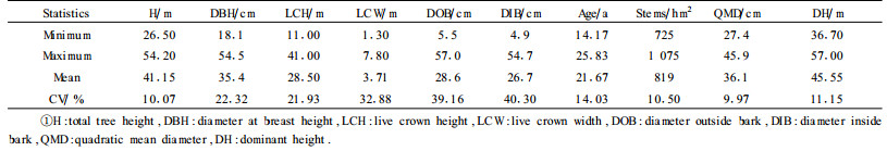
Fig. 1A shows the plot of the relative diameter over the relative height of trees with diameter at breast height bigger than 40 cm and of trees with a diameter at breast height less than 30 cm. Fig. 1B presents the relative form using a moving average model with respect to diameters of both data sets. There are differences in stem form(Fig. 1A), but these are difficult to interpret. It can be seen that there is no influence of diameter at breast height on stem form(Fig. 1B). This stem form variation can partly be attributed to the effect of height/diameter at breast height ratio [h/d-ratio](Fig. 2A). The trees with a h/d-ratio exceeding 1.4 show a higher relative diameter below 50 percent of their total height. The trees with a low height diameter ratio are characterized by a pronounced butt sweep. In comparison with other studies, Schmidt(2000) found that the tree dimensions and h/d-ratio had a clear influence on stem form ofNorway spruce.

Fig. 2A shows the plot of relative diameter over the relative height of trees with h/d-ratio greater than 1.4 and of trees with a h/d-ratio less than 1.0. Fig. 2B presents the relative form with respect to h/d-ratios of both sets of trees.

3 Methods

Two parameter-parsimonious taper functions were used for developing stem taper models for Eucalyptus trees, the modified Brink function and the Pain function. A two stage procedure is used to develop the models. In the first stage the parameters of the taper functions(4, 5) were estimated for each tree. Secondly attempts were made to establish relationships between single tree function parameters and tree or stand variables. The theory of both functions is discussed in the following sections.

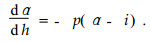
3.1 The modified Brink function

Based on the assumption that an ideal form of a tree stem is composed of two parts, an upper part and a lower one, Brink et al.(1986) developed differential equations for the description of a tree stem profile. The differential equation for the lower stem part is:

(1)

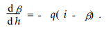
The equation defines the rate of change of the radius dα as a function of change of the height dh which is proportional to the difference between the radius α and an asymptotic radius i. The equation for the upper part is as follows:

(2)

Where β is the stem radius. The following three-parameter function for the whole profile was developed from(1) and(2):

(3)

Where, r(h):tree radius(cm) at height(m), H:total tree height(m), r_1.3:tree radius at breast height, i:parameter(common asymptote), p:parameter(describing lower part of stem), q:parameter(describing upper part of stem).

The three parameters describe different stem parts and therefore, they may be assumed to have some biological meaning. The parameter i is equal to the asymptotic value, which would be reached by both exponential functions at height ∞ and-∞. The height(h) with radius i describes the position between two differently shaped stem sections. The parameter p describes the external(left) bending of the stem curve in the lower stem part, while q describes the internal(right) bending in the upper stem part(Brink et al., 1986; Hui, 1997; Riemer et al., 1995).

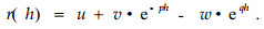
r(h) should be equal to zero, when h=H. This secondary requirement was not fulfilled by the original equation(3). Therefore Riemer et al.(1995) proposed the following modified function:

(4)

Where,

The symbols used in equation(3) are also valid here.

Fig. 3 shows the three parts(u, v·e^-p·h, w·e^q·h) of the Brink function describing a stem form of a tree with DBH 34.4 cm which is the average value of the data set and height of 44.4 m. The average parameter values of the whole data set of 153 trees were used.

3.2 The Pain function

Pain et al.(1996) developed a taper model using data collected from even-aged Norway spruce grown in France. In comparison to the modified Brink function, the Pain function requires a two stage procedure because stem diameter is only determined as a function of relative height. A second step is necessary to consider tree dimensions. An evaluation is made to see whether the function considers the existing tree form differences or only differences in tree dimensions. The modified Brink function also requires a two stage modeling procedure if a stand or a generalized taper model should be developed instead of a model with average parameters. The Pain function reads as follows:

(5)

Where, d_i:diameter over bark at height h_i=h_rr×total tree height, h_r:relative height from ground, 0≤h_r≤1, α, β:parameters.

In the second stage the parameters α and β were related to individual tree variables using regression equations:

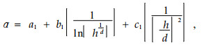
(6)

(7)

Where, a₁, b₁, c₁, a₂, b₂, c₂:parameters, h: height(m), d:diameter at breast height(cm).

Fig. 4 presents the Pain function describing the stem of the average tree with a DBH of 34.4 cm.

3.3 Parameter prediction of the modified Brink function

An attempt was made to develop a model for the description of variation in stem form with the help of the modified Brink function(4). As shown in Fig. 1 and 2 there is a small variation in stem form which may be explained by h/d-ratio of a tree. Hui(1997) determined the i parameter as a function of the diameter at breast height, the q parameter as a function of total tree height and the quadratic mean diameter and the p parameter is related to quadratic mean diameter. Based on these findings, attempts were made to establish relationships between model parameters and tree and stand variables. In agreement with Hui(1997) the parameter i may be estimated as a function of breast height diameter, as follows:

(8)

Relating the parameter q to dominant height proved to be more suitable in our data set:

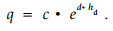
(9)

The parameter p could be determined as a function of quadratic mean diameter:

(10)

Where, DBH:diameter at breast height(cm), h_d:dominant height(m), d_q:quadratic mean diameter(cm), i:parameter(common asymptote), p:parameter(describing lower part of stem), q:parameter(describing upper part of stem), a, b, c, d, f:parameters.

Substituting equations(8), (9) and (10) in equation(4) could develop a general stem model for the description of the stem profile of Eucalyptus grandis. The model parameters were estimated with the help of non-linear regression using the available database(a=0.555 224; b=0.935 585; c=0.064 744; d=-0.010 402; f=-14.770 149).

The coefficient of determination(R²) of the parameter i is equal to 0.78. The coefficients of determination of the q and p parameter estimates are approximately zero(0.03 and 0.01 respectively). An R²-value of zero means that the fit is no better than the mean. Thus most probably the parameter prediction model makes no improvement in comparison to an average parameter model.

3.4 Average parameter estimates of the modified Brink function

The available data shows that there is a weak relation between q and p parameters and the stand variables. Therefore, the mean values of q and p for the whole data set were estimated to test if the first model improved the predictability of stem radius compared to that model with a mean value of q and p. The second model was developed by substituting equation(8) in equation(4). For this model the parameter values were a=0.577 426; b=0.924 790; q=0.039 704; p=0.657 624.

3.5 Parameter prediction of the Pain function

The parameters α and β were estimated two times. The first estimates were obtained by fitting the data of each tree to equation(5). The coefficients of the regression equations(6) and (7) were calculated by fitting the data sets of α and β using diameter at breast height(d) andheight(h) of each tree as independent variables(R²=0.86 and 0.61, for α and β, respectively). The coefficients of the regression equations were a₁=-5.298 622, b₁=3.687 900, c₁=-10.150 884, a₂=-0.486 671, b₂=-0.737 463, c₂=-0.298 816. Then the parameters α and β of the model were predicted as a function of diameter at breast height and total tree height.

The assumption that the parameter prediction model can describe trees of different stem forms was tested. For this purpose parameters were estimated for relative model forms by using relative diameter, defined as stem diameter over maximum stem diameter, instead of absolute diameters on the left hand of the function. Using relative variables instead of absolute variables reduces every tree to its actual form independent of its dimension. No relationship could be established between the parameters of the relative model form(α_rel, β_rel) and the h/d-ratio(R²=0.01 and 0.03, for α_rel and β_rel, respectively). Also there is no relation between α_rel and diameter at breast height(R²=0.00) and a weak relationship between β_rel and diameter at breast height(R²=0.10). As shown in Fig. 2B the h/d-ratio variable has a small influence on stem form. This may indicate that the model is not suitable for describing differences in stem forms. But this may be due to the fact that the available data set contains a narrow range of h/d-ratios. Schmidt(2000) showed that for Norway spruce the effect of h/d-ratios of less than 0.9 is greater than the effect of h/d-ratios over 1.0. Trees with low h/d-ratio representing wide initial spacing and heavy thinning are not part of the data set and thus the influence of a low h/d-ratio cannot be evaluated. The influence of tree size on taper form, which was considerable in Norway spruce trees, does not show in the Eucalyptus grandis data set. A problem always appearing is the correlation between function parameters that overlay the relationship between form describing function parameters and parameter prediction variables.

Fig. 5 presents the plot of the parameter α_rel and β_rel overdiameter at breast height.

The plots of the parameter α_rel and β_rel of the Pain function over the tree h/d-ratios.

4 Evaluation of the models

The models were evaluated using the mean residual and the root mean square error using the following formulae:

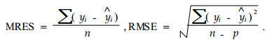
Where, MRES:mean residual, RMSE:root mean square error, y_i:observed value; :predicted value, n:number of data pairs; p:number of model parameters.

An evaluation of the two Brink functions revealed that the model with average parameter values and the model with predicted parameters estimated the over-bark radius of the 153 trees with similar accuracy. A root mean square error of 0.68 cm and 0.67 cm was obtained for the average parameter model and the predicted parameter model, respectively. Thus it was decided to compare the model with the mean parameter values with the Pain function.

The average bias and the root mean square error were calculated for ten relative height classes. The mean biases in different relative height classes vary from-0.27 to 0.38 cm for the Brink model and from-0.31 to 0.35 cm for the Pain function. The root mean square error ranged from 0.45 to 0.74 cm and from 0.41 to 0.77 cm for the Brink function and the Pain function, respectively.

Fig. 6A shows that both models underestimate stem radius of the lower and the upper third of the stem and overestimate stem radius in the middle stem part. Fig. 6B shows that the two models estimate the stem radius with approximately equal accuracy.

The root mean square errors were also calculated for trees having different h/d-ratios in order to see the response of the models in estimating the stem radius of extreme trees. The h/d-ratio of all measured trees ranges from 0.8 to 1.8. The two models estimated the stem radius of trees with different h/d-ratios with approximately equal accuracy(Fig. 7). Both models predicted the stem radius of trees with h/d-ratio greater than 1.0 more accurately than trees with h/d-ratio equal or less than 1.0.

5 Discussion and conclusions

Three taper models were evaluated using Eucalyptus grandis stem data. Two models are based on the modified Brink function and the third on the Pain function. The stem form could be described with high accuracy for both the modified Brink function and the Pain function. An attempt to generalize the model using tree and stand variables failed. This may be due to the rather narrow range of dominant heights(36.70~57.00 m), quadratic mean diameters(27.4~45.9 cm) and stand densities(725~1 075 stems·hm^-2).

The generalization approach followed by Hui et al.(1997) should be pursued using the Brink function with a more comprehensive data set, covering a wider range of stand densities and heights. The Pain function was parametrized by relating the parameters(α and β) to diameter at breast height, total tree height and h/d-ratio. But in the Eucalyptus grandis data set the model could not describe differences in stem taper of individual trees.

In consequence, because the existing differences in taper cannot be explained by single tree or stand variables(Fig. 1, 2), both models can be used only for predictions of average stem taper, which is the usual practice. Fig. 2B shows only minor differences in tree form for different h/d-ratios which the model is not able to describe. Also, in contrast to previous work in spruce trees, tree size has no effect.

The results of this study can be summarized as follows:

1) The stem profile of a tree can be described with sufficient accuracy, using a variety of parameter-parsimonious taper functions, two of which were presented in this paper.

2) The major challenge of using a parameter-parsimonious taper function lies in its potential for generalization, i.e. for predicting stem form as a function of individual tree characteristics as well as stand density, stand height and site using parameter prediction(Bi, 2000; Pain et al., 1996; Real et al., 1987).

3) The modified Brink function is in principle suited for this purpose, as was shown by Hui et al.(1997) for a large data set of Cunninghamia lanceolata. Our Eucalyptus grandis database was not sufficient for achieving a similar success. Thus further studies with a more comprehensive data set, covering a wide range of tree dimensions and stand densities, are recommended.

4) It was possible to relate the parameters of the Pain function to tree variables(height, DBH). This is not surprising because absolute diameter is predicted from relative height in the original Pain function. Differences in stem form could not be detected when using relative diameters. This may be due to the specific data set. In principle, the Pain function should be suitable for developing a generalized taper model.

5) The Pain function should be made compatible by constraining the model radius at breast height such that it is identical to the observed one, but this may be achieved at the cost of reduced flexibilty.