1   Introduction

Carbon capture and storage (CCS) is a promising approach to mitigating global warming, and among the available carbon sequestration technologies, geological sequestration is considered the most effective (Zhang et al., 2023). In particular, marine CO₂ geological storage has great potential, accommodating about 40% of the CO₂ storage capacity (Li et al., 2023). China's saline water layer is widely distributed and has a large area, with its theoretical CO₂ storage accounting for over 95% of the geological utilization and theoretical storage capacity in the country (Li et al., 2022). However, in conducting carbon sequestration, the potential leakage risk in the CO₂ reservoir is the most worrying problem; once it is leaked, it may have serious impacts on biodiversity, the ecological environment, and the entire marine environment (Kim and Park, 2023). Therefore, CO₂ plume migration and potential leakage detection are important. Although leak detection can be a major risk, plume boundaries must be monitored and storage levels verified throughout the process.

Recent studies have found that the seismic wave velocity used in traditional methods does not change significantly with CO₂ saturation upon exceeding a certain limit, posing challenges to plume migration monitoring in CO₂ sequestration (Bhuyian et al., 2012). In the deep saline water layer, the rock layer with high porosity and high permeability is filled with saline or saline water, which increases the total resistivity of the deep saline water layer (Fawad and Mondol, 2021; Li et al., 2013). With the continuous injection of CO₂ and the migration of supercritical CO₂ plumes, a high-resistivity response appears locally in the deep saline water layer (Fawad and Mondol, 2021). Among these, the controllable source electromagnetic method (CSEM) has a significant response to the resistivity change caused by CO₂ saturation and has an effect on the response of medium and high saturation (Eide and Carter, 2020). As CSEM works in the frequency domain and has the advantage of having strong anti-interference ability and high signal-to-noise ratio, it can analyze the resistivity distribution of submarine strata by receiving reflected and refracted electromagnetic signals from submarine strata Compared to seismic monitoring, CSEM monitoring has a lower cost and can better meet the needs of long-term monitoring and the safety, effectiveness, and economic requirements of geological carbon sequestration.

Despite its advantages in monitoring CO₂ injection and migration, only a few studies have investigated the use of CSEM for CO₂ sequestration monitoring. By using a modified secondary field method, one study addressed the airwave problem occurring when CSEM is applied to a target beneath a shallow sea (Kang et al., 2012). Du and Nord (2012) investigated the sensitivity of the CSEM to buried thin resistive layers that could represent CO₂ storage reservoirs. This study first investigated the sensitivities of three-dimensional (3D) CSEM data to a realistic CO₂ storage and then analyzed the use of CSEM data for making estimates of the post-injection build-up of CO₂ layers in the subsurface. Vilamajó et al. (2013) evaluated the ability of the CSEM to monitor CO₂ storage at the Research Laboratory on Geological Storage of CO₂ at Hontomín located in Burgos, Spain. The synthetic time-lapse study explored the possibilities of CSEM monitoring with a deep electric source. Park et al. (2017) revisited the marine CSEM data and acquired the Sleipner CO₂ storage to further study the dataset, demonstrating the feasibility of marine CSEM for offshore CCS monitoring. Similarly, the current study confirms that marine CSEM can be an important tool for offshore CO₂ storage monitoring. Meanwhile, Puzyrev (2019) explored the potential of using deep learning methods for electromagnetic inversion. This method's performance was assessed using models of strong practical relevance representing an onshore controlled source electromagnetic CO₂ monitoring scenario.

Furthermore, Ayani et al. (2020) presented a stochastic optimization method called the "ensemble smoother" to invert time-lapse marine-controlled source electromagnetic data for predicting the CO₂ plume location. The results obtained after the inversion of electromagnetic data show that the proposed method can accurately predict CO₂ plume location and quantify the associated uncertainties. Fawad and Mondol (2021) dealt with the CO₂ plume delineation and saturation estimation using a combination of seismic and electromagnetic synthetic data. The results revealed that monitoring the CO₂ plume in terms of extent and saturation is feasible either using repeated seismic and electromagnetic data or combining baseline seismic data with repeated electromagnetic data. Tveit et al. (2020) explored the application of CSEM or gravity and seismic acoustic amplitude inversion (AVO) in monitoring large-scale carbon dioxide injection processes. The current version of the simulation modeling problem in CCS work has also become relatively mature. For example, the stage-based modeling capability in Sim CCS is particularly useful for optimizing the dynamic deployment of CCS projects (Ma et al., 2023), along with other simulation modeling methods, thus proving the feasibility of simulation modeling methods.

The current study evaluates the sensitivity of CSEM to monitor the process of plume transport in offshore CO₂ storage. First, we established a numerical simulation model for CO₂ plumes during storage and determined the geometric shape and characteristics of the monitoring area. Then, we used CSEM to numerically calculate the electromagnetic field response of the simulation model, after which we analyzed the sensitivity of different parameters to the electromagnetic field response. Doing so provides a theoretical and practical basis for further research into and the application of CSEM, which is of great significance for improving the safety and stability of offshore CO₂ storage.

2   Identifying CO₂ plume CSEM method

2.1   CSEM soundings

CO₂ stored in the seabed typically exhibits higher electrical resistivity than surrounding media. Electromagnetic detection is sensitive to formation resistivity; thus, it is considered the best method for deep fluid identification. The principle of CSEM soundings is to use electromagnetic induction phenomena, in which the alternating current (AC) electric field can induce the AC magnetic field, which, in turn, can also induce the AC electric field. Therefore, energy is constantly converted in the form of electric and magnetic fields and radiates into space through the alternating radiation between the two fields. The same refraction and reflection occur when it encounters different media interfaces.

When electromagnetic fields propagate in media with different levels of resistivity, they have both similar and different characteristics. On the one hand, the similarity lies in the fact that the energy of electromagnetic waves will decrease in a geometric attenuation manner as the propagation distance increases, regardless of whether the medium has high or low resistivity. On the other hand, the difference can be attributed to the high-resistivity media hardly absorbing the energy of electromagnetic waves, while low-resistivity media strongly absorb the energy of electromagnetic waves, implying the occurrence of an eddy current. Therefore, the received electromagnetic field response can be analyzed to obtain the electrical distribution of the underground medium.

In Figure 1, a 2D measurement grid consisting of multiple measurement lines can be used for 3D exploration. The ship towed a long cable with an HED transmitter near the seabed to enhance the weak response signal below. The transmitter emits low-frequency electromagnetic waves with controllable waveforms. Waves propagate to the surrounding areas, resulting in the following: 1) penetration of the seabed strata received by the receiver (red line), 2) propagation in the seawater received by the receiver (yellow line), and 3) propagation through the seabed (blue line). If the receiver can measure a clear electromagnetic response signal of CO₂ plumes, it can help detect the distribution of the CO₂ plume transport.

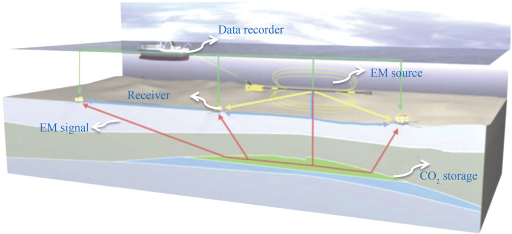Figure  1  Configuration of the marine CSEM exploration system, including a near seafloor deep-towed horizontal electric dipole (HED) transmitter and multiple seabed receiver arrays arranged along the survey line

Download: Full-Size Img

Here, we assume that the electrical conductivities of air, seawater, submarine sediment, and HC are σ_air, σ_water, σ_sed, and σ_r respectively; the magnetic permeability in the earth is the distance of the current source from the seafloor is h_c, the thickness of the seawater layer is h_w, the depth below the seafloor of the top of HC is h_r, and the time factor is e^−iωt. Thus, the system of classical Maxwell's equations yields the following:

where J_i denotes the current density of the excitation source term, ε is the dielectric constant, and ω is the angular frequency. In considering the IP effect, we should also include the polarization current term. Thus, by the derivation of Harrington (1961), Eq. (2) above can be written as follows:

where J_s = (σ_r − σ_sed) E, and J_s denotes the polarization current within the target body. Taking the curl on both sides of the equal sign of Eq. (1), simultaneously, the curl of the magnetic field is substituted into Eq. (3) and then simplified to obtain the fluctuation equation containing only the electric field vector as follows:

The electric field E in Eq. (4) contains the incident and scattered fields; thus, E = E_i + E_s, and from this, it can be shown that the electric field of the two parts satisfies the equation.

In solving for the scattered field, which is deemed an ordinary current source, we refer to the theory of Dyadic Green's function (Tai, 1994). As such, integration over the target body leads to the following:

Based on the method of integral equations combined with the theory of DGF, the following integral equations are obtained by transforming and simplifying Eqs. (1) and (2):

where E_i (r) is the incident field excited by the transmitted source in accordance with the classification made by Tai (1971), and G(r|r') is a category-Ⅲ DGF.

Using Eq. (7) in the case where in the incident field (i.e., primary field) E_i (r)has been solved, it is possible to calculate the electric field at each point within the anomaly. As such, the electric field at each point in the model can then be calculated from the corresponding DGF.

The 3D target body is dissected into n small cells while assuming that the electric field inside each dissected cell is constant and equal to the electric field at its center. Hence, Eq. (3) can be written as follows:

Thus, the following expression for the electric field at the center of the mth cell is obtained:

where $\boldsymbol{\varGamma}_{m n}=\int\limits_{V_A} \boldsymbol{G}\left(r \mid r^{\prime}\right) \mathrm{d} v^{\prime}$. Based on Eq. (9), the matrix equation is obtained as follows:

where $\boldsymbol{\delta}_{m n}= \begin{cases}\boldsymbol{I}_{m n} & m=n \\ \boldsymbol{\theta}_{m n} & m \neq n\end{cases}$, I is the unit dyadic.

Occam inversion using MARE2DEM code. The Occam inversion algorithm is a least squares method based on the regularization idea, and its objective function is to minimize the following unconstrained optimization problem:

where m is the n-dimensional model parameter vector, R is the roughness operator, and μ is a regularization operator, which is used to balance the roughness and poor fitting of the data. If μ is larger, the inversion result tends to be smooth; otherwise, it tends to fit the data. In addition, W is the diagonal weighting matrix for the fit difference, d is the observation data vector, and F(m) is the forward response corresponding to model m.

Finally, the roughness of the model can be expressed as follows:

where λ is the anisotropic penalty term, $\boldsymbol{m}^{\prime}=\left[\begin{array}{lll} \boldsymbol{m}_{\boldsymbol{y}} & \boldsymbol{m}_z & \boldsymbol{m}_x \end{array}\right]^{\mathrm{T}}$.

For the kth iteration model, the iteration in which the objective function is sufficiently reduced takes the following form:

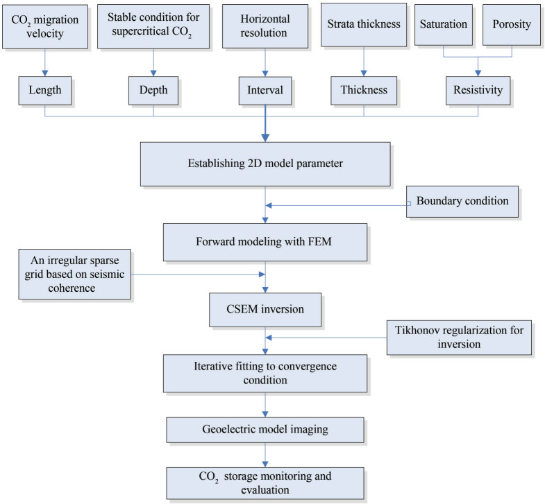Figure  2  Flow chart of the CSEM for identifying the plume migration of offshore CO₂ storage

Download: Full-Size Img

where the difference vector is fitted $\hat{d}=\boldsymbol{d}-F\left(\boldsymbol{m}_k\right)$.

In the present study, we applied the finite element unstructured mesh method to two-dimensional (2D) electromagnetic fields forward modeling. We used the irregular triangular mesh instead of the traditional rectangular mesh, which is more in line with complex structural boundaries, thus saving a considerable amount of computing memory and greatly improving computing efficiency and accuracy (Wen and Benson, 2019). At the same time, the mesh with insufficient precision is refined through continuous iteration, thus ensuring calculation accuracy.

2.2   Identifying plume migration using CSEM

The migration of CO₂ plumes in seabed geological storage refers to a special flow pattern formed in underground reservoirs as a result of the injection of carbon dioxide and the migration of underground fluids. Its characteristics include high flow velocity, large diffusion coefficient, and short transport distance. The ocean CSEM is commonly used to monitor the path and velocity of plume transport in the ocean by measuring changes in the electromagnetic field. Due to its high flow velocity and plume transport diffusion coefficient, the ocean CSEM has better sensitivity and analytical ability compared to traditional monitoring methods.

2.3   CO₂ saturation calculation formulas

We used the Archie equation to calculate water saturation in marine sediments (Archie, 1942). In a reservoir, the filling of sedimentary layers can be approximated as the filling of CO₂ and seawater, and this is expressed in the following equation:

where B is the equivalent cation conductance, which is dependent on temperature and salinity, and Q_v is the cation exchange capacity per unit volume.

Then, isolating ρ_t, we obtain:

where ϕ_sh is the total shale porosity, and ρ_sh is the resistivity of the formation with 100 percent volume of shale (V_sh), while m and a are the cementation and tortuosity exponents for the clay-rich formation, respectively.

In this paper, we assumed the following values: rock porosity (ϕ) = 0.2, cementation index (m) = 1.6, tortuosity coefficient a = 1.1, saturation index (n) = 1.8, CO₂ saturation S_w = 0.5, pore fluid resistivity (ρ_w) = 0.2, ρ_sh = 0.4 Ω⋅m, seawater resistivity ρ_w = 0.3, and total shale porosity ϕ_sh = 0.3 (Harp et al., 2019; Yilo et al., 2023).

3   Experiments

Meanwhile, we have considered various potential scenarios for the migration and diffusion of offshore CO₂ storage (Hoffman and Alessio, 2017), including various burial depths, lateral extension diffusion, vertical extension diffusion, electric field components, and multiple combinations of lateral intervals. The models include the following: 1) various lengths of lateral diffusion, 2) burial depths, 3) spacing of lateral diffusion, 4) thickness of vertical diffusion, and 5) saturation models.

Based on the formula derivation calculation, we set the resistivity of the CO₂ model in this experiment as 100 Ω. The model parameter settings used in this study are shown in Table 1.

3.1   Various electric field components

In this group of experiments, we conducted a comparative analysis of the difference in the response amplitudes of E_x, E_y, and E_z when there is no abnormal object in Model 1-4. Then, we compared the abnormal response characteristics under different components.

We conducted forward modeling without a CO₂ plume and calculated the response values of each component of the electromagnetic field detected by CSEM at five different frequencies of the corresponding blank field. Next, we generated the amplitude of the difference in response between the blank field and each component under the response of the target body. Normalized anomaly amplitudes were plotted for three electric field components (E_x, E_y, and E_z) calculated at identical frequencies (0.25 Hz) (Figure 3).

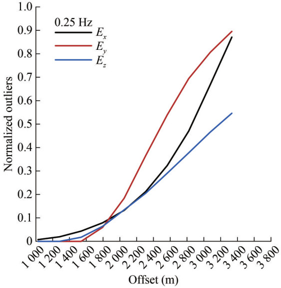Figure  3  Normalized anomalous amplitude response (sensitivity) of three electric field components (E_x, E_y, and E_z) using the transmitted frequency = 0.25 Hz for Model 1-4

Download: Full-Size Img

By comparing and analyzing the normalized anomaly amplitude curves of the three electric field components in Figure 3, it can be clearly seen that the three electric field components can obtain a good anomaly response to the detection target. In particular, the E_y component increases with the offset, and the abnormal response characteristics of the electric field obtained are the most obvious than for the E_x and E_z components. This means that the abnormal amplitude signal obtained under the measurement of the E_y component is the strongest and easiest to observe, and that of the E_z component is the weakest; that is, the abnormal signal observed under the measurement of this component is weak and difficult to observe.

The normalized anomaly amplitudes of E_x electric field components at five different frequencies (0.25, 0.75, 1, 3, and 5 Hz) were also plotted (Figure 4).

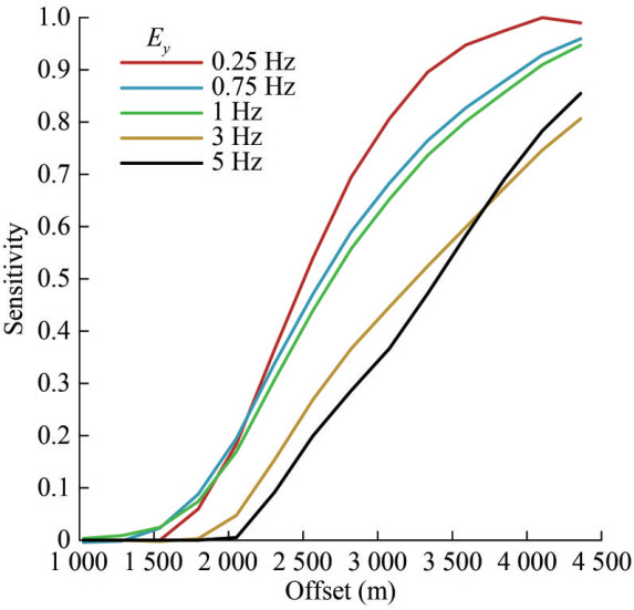Figure  4  Normalized anomalous amplitude response (sensitivity) of the E_y electric field vs. offset using five transmitted frequencies = 0.25, 0.75, 1, 3, and 5 Hz for Model 1-4

Download: Full-Size Img

By comparing and analyzing the normalized anomaly amplitude curves of the E_y electric field components in Figure 4, it can be clearly seen that the E_y component can obtain a good and stable abnormal response signal under the five measured frequencies, and the strength of the abnormal response signal changes regularly with the frequency. When the lower frequency increases from 0.25 Hz to the higher frequency of 5 Hz, the abnormal response signal obtained at the same offset is gradually weakened. In other words, the electric field abnormal response signal at 0.25 Hz is the strongest, while the relative abnormal response signal at 5 Hz is the weakest.

3.2   Various lengths of lateral diffusion

Transverse diffusion is the main mode of CO₂ plume migration because the heterogeneity of horizontal reservoirs tends to limit the vertical migration of CO₂ (Hoffman and Alessio, 2017), and most of the supercritical CO₂ plumes will gather under the sealing layer and migrate in the form of thin layers with high gas saturation. Meanwhile, when the plume permeability contrast is greater than 50, supercritical CO₂ flows only in the highly permeable layer.

In the proposed model, we adopted the simulated burial depth of 800 m based on previous studies, which reported that if the burial depth in the offshore geological storage engineering is too deep, it will increase the economic cost and implementation difficulty of the project (Guo et al., 2015). One study concluded that the burial depth of 800 m has met the temperature and pressure conditions required for CO₂ to be a supercritical state (Zendehboudi et al., 2011). Meanwhile, we also refer to the Enping Project, the first offshore CO₂ storage project in China, in which the point of burial is also a saltwater layer located 800 m below the sea floor.

We used models of varying lengths (Models 1-1, 1-2, 1-3, and 1-4) for the lateral diffusion of offshore CO₂, enabling us to evaluate the CSEM's ability to distinguish CO₂ lateral diffusion. The corresponding CSEM resistivity imaging results are shown in Figures 5(e)–(h). As shown in the figures, the high-resistivity range and high saturation range obtained from imaging are consistent with the reservoir range of the model. The model parameters are shown in Table 3.

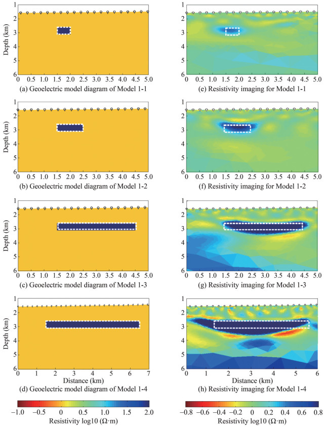Figure  5  Electrical resistivity imaging of lateral migration at various intervals in the offshore CO₂ storage for Models 1-1, 1-2, 1-3, and 1-4

Download: Full-Size Img

The length of the high-resistivity area basically corresponds to the length range of the lateral extension and diffusion of offshore CO₂. However, significant differences are also observed in the inversion results of offshore CO₂ (Models 1-1, 1-2, 1-3, and 1-4) with varying ranges of lateral diffusion. In Model 1-1, the top inversion depth and regional range of the offshore CO₂ storage are closest to the simulated depth and regional range. Meanwhile, in Models 1-2, 1-3, and 1-4, as the lateral diffusion range of offshore CO₂ gradually lengthens, the imaging depth and regional range of the offshore CO₂ storage gradually deviate from the simulated model. However, overall, the approximate range of the model can still be obtained to determine the approximate position of the target body.

Regarding the inversion of Model 1, the curve of the RMS misfit and roughness change with the number of iterations is shown in Figure 6.

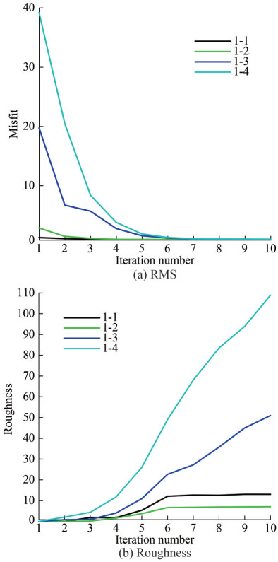Figure  6  RMS and roughness curve inversion with iterations of Models 1-1, 1-2, 1-3, and 1-4, respectively (Black, green, blue, light blue)

Download: Full-Size Img

Figures 5(a)‒(d) are schematic diagrams of Models 1-1, 1-2, 1-3, and 1-4, respectively; Figures 5(e)‒(h) represent resistivity imaging for Models 1-1, 1-2, 1-3, and 1-4, respectively. In Figures 5(a)‒(d), dark blue represents the range of offshore CO₂ diffusion areas, light yellow represents marine sediments, and black boxes represent offshore CO₂ reservoirs.

As shown in Figure 6, the roughness increases with the increase of iterations. Furthermore, the RMS misfit of Occam inversion converges with the increase of iterations, and the target misfit is 1. The inversion RMS misfit of the four models all reach the target misfit in the 7th iteration, there by proving that the inversion results are reliable. The comparison between the inversion data of Model 1-1 and the actual target body data is shown in Figure 7.

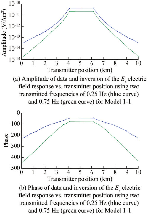Figure  7  Amplitude and phase of data and inversion of the E_y electric field response vs. transmitter position using two transmitted frequencies of 0.25 Hz (blue curve) and 0.75 Hz (green curve) for Model 1-1

Download: Full-Size Img

Upon comparing the error range of the inversion target body of different models under two frequencies, namely, 0.25 Hz (blue curve) and 0.75 Hz (green curve), we found certain differences between the inverse resistivity value and the real value. However, there is little difference between the inversion results of the two models and the actual object, and the error range is relatively stable.

3.3   Various burial depths

In the proposed model, we used three different burial depths of 1 000, 1 500, and 2 000 m for discussion. These represent the main burial depths of saltwater reservoir sequestration projects that have been implemented around the world. The major ones include the 1 000 m burial depth adopted by the Sleipner project in Norway (Czernichowski-Lauriol et al., 2003), the 1 500 m burial depth adopted by the Ordos Project in China, and the 2 000 m burial depth by the Gorgon project in Australia (Flett et al., 2009).

Furthermore, we used various burial depth models for offshore CO₂ plumes (Models 2-1, 2-2, and 2-3) to evaluate the CSEM's ability to distinguish the burial depths of offshore CO₂ plumes. The corresponding resistivity imaging results from CSEM are shown in Figures 8(d)‒(f). The high-resistivity range and high saturation range obtained from imaging are consistent with the plume range of the model. The model parameters are shown in Table 4.

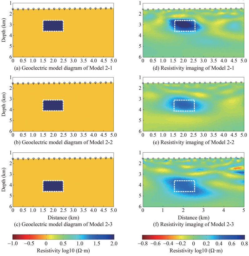Figure  8  Electrical resistivity imaging of lateral migration at various intervals in the offshore CO₂ storage for Models 2-1, 2-2, and 2-3

Download: Full-Size Img

Figures 8(a)‒(c) are schematic diagrams of Models 2-1, 2-2, and 2-3, with dark blue indicating the range of offshore CO₂ diffusion areas, light yellow indicating marine sediments, and white boxes indicating offshore CO₂ reservoirs; Figures 8(d)‒(f) are resistivity imaging of Models 2-1, 2-2, and 2-3, respectively.

The inversion results in the figure all show that the four models have begun to converge to the vicinity of the real model after the 10th iteration, indicating that the inversion method is real and effective. Furthermore, the depth of the high-resistivity region basically corresponds to the depth range of offshore CO₂ storage and burial. However, the inversion results of these models are still different. Among these, the inversion depth and area range of offshore CO₂ storage in Model 2-1 are the closest to the depth and area range simulated by the model. In Models 2-2 and 2-3, the inversion depth and regional range of offshore CO₂ sequestration gradually deviate from the simulated model as the simulated depth increases. However, the overall range of the approximate model can still be determined to determine the approximate target location.

For the inversion of Model 2, the curve of the RMS misfit and roughness change with the number of iterations is shown in Figure 9.

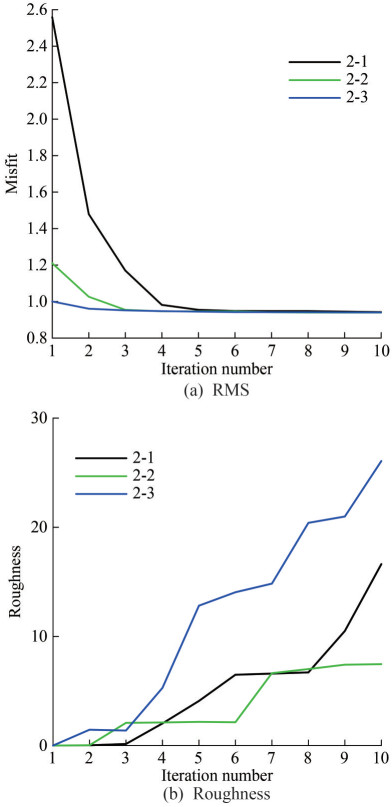Figure  9  RMS and roughness curve inversion with iterations of Models 2-1, 2-2, and 2-3, respectively (Black, green, blue)

Download: Full-Size Img

As shown in Figure 9, roughness increases with the increase of iterations. Furthermore, the RMS misfit of Occam inversion converges with the increase of iterations, and the target misfit is 1. The inversion RMS misfit of all four models can reach the target misfit in the 6th iteration, there by proving that the inversion results are reliable. The comparison between model inversion data and actual target data is shown in Figure 9.

The curves from top to bottom correspond to Models 2-1, 2-2, and 2-3, respectively (Figure 10). We compared the error ranges of the inversion target body of different models at two frequencies of 0.25 Hz (blue curve) and 0.75 Hz (green curve) and found certain differences between the inverse value of the resistivity and the real value. However, the inversion results of the three models had little differences with the actual target body, and the error ranges of the inversion increased with the increase of the burial depth. Nevertheless, the margin of error is stable.

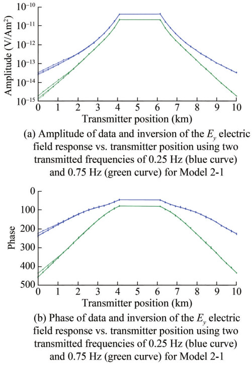Figure  10  Amplitude and phase of data and inversion of the E_y electric field response vs. transmitter position using two transmitted frequencies of 0.25 Hz (blue curve) and 0.75 Hz (green curve) for Model 2-1

Download: Full-Size Img

3.4   Various spacing of lateral diffusion

We used various spacing lateral diffusion models for offshore CO₂ plumes (Models 3-1, 3-2, 3-3, and 3-4) to evaluate the CSEM's ability to distinguish the various spacing lateral diffusions of offshore CO₂ plumes. The corresponding resistivity imaging results from CSEM are shown in Figures 11(e)‒(h). The high-resistivity range and saturation range obtained from imaging are consistent with the plume range of the model. The model parameters are shown in Table 5.

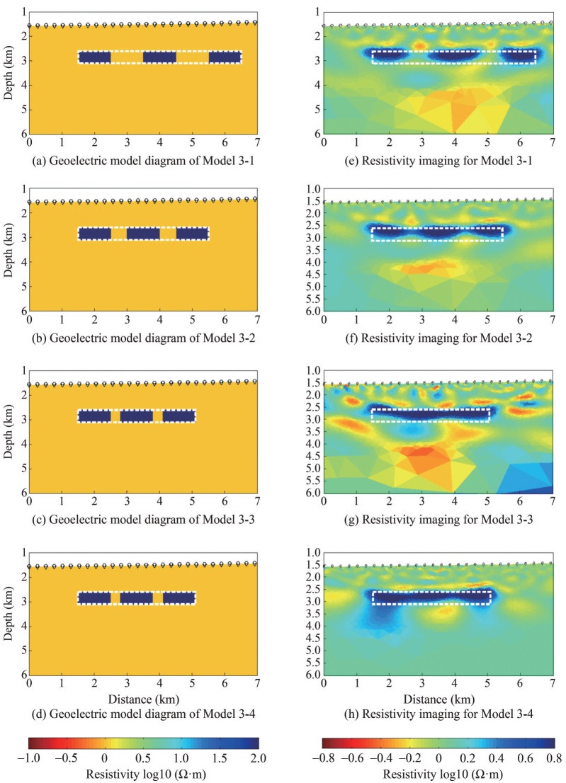Figure  11  Electrical resistivity imaging of lateral migration at various intervals in the offshore CO₂ storage for Models 3-1, 3-2, 3-3 and 3-4

Download: Full-Size Img

Figures 11(a)‒(d) are schematic diagrams of Models 3-1, 3-2, 3-3, and 3-4, with dark blue indicating the range of offshore CO₂ diffusion areas, light yellow indicating marine sediments, and white boxes indicating offshore CO₂ reservoirs; Figures 11(e)‒(h): Electrical resistivity imaging of Models 3-1, 3-2, 3-3, and 3-4.

Although the depth of high-resistivity areas basically corresponds to the burial depth range of offshore CO₂, reservoirs, differences can still be observed in the inversion results of the four different models (Figure 11). Among these, the inversion depth of the offshore CO₂ storage in Model 3-1 is closest to the depth simulated by the model and the range and boundary of the regional target body area. In Models 3-2, 3-3, and 3-4, there is a slight deviation between the inversion depth and regional range of the offshore CO₂ reservoir, along with the boundary and the simulated model, as the simulated distance between adjacent target bodies decreases. The intermediate boundary of adjacent target bodies cannot be determined based on the inversion image. However, the range of the overall model can still be determined to determine the approximate position of the target body.

For the inversion of Model 3, the curve of RMS misfit and roughness change with the number of iterations is shown in Figure 12.

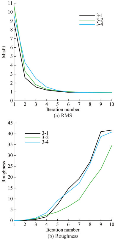Figure  12  RMS and roughness curve inversion with iterations of Models 3-1, 3-2, and 3-4, respectively (Black, green, blue)

Download: Full-Size Img

As shown in Figure 12, the roughness increases with the increase of iterations. Furthermore, the RMS misfit of Occam inversion converges with the increase of iterations, and the target misfit is 1. The inversion RMS misfit of all four models can all reach the target misfit in the 7th iteration, thus proving that the inversion results are reliable. The comparison between model inversion data and actual target data is shown in Figure 13.

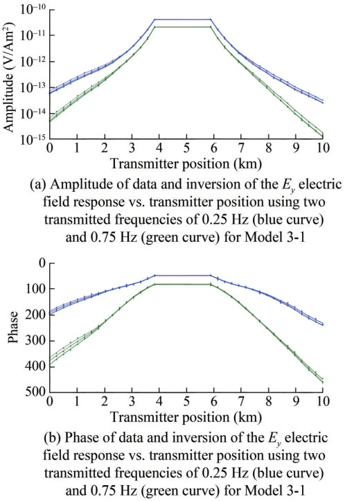Figure  13  Amplitude and phase of data and inversion of the E_y electric field response vs. transmitter position using two transmitted frequencies of 0.25 Hz (blue curve) and 0.75 Hz (green curve) for Model 3-1

Download: Full-Size Img

The curves from top to bottom correspond to Models 3-1, 3-2, and 3-4, respectively (Figure 13). Upon comparing the error ranges of the inversion target bodies of different models at two frequencies of 0.25 Hz (blue curve) and 0.75 Hz (green curve), we find differences between the inversion values of resistance and the real values. However, there is little difference between the inversion results of the four models and the actual target bodies. Furthermore, the error ranges of inversion also increase with the increase of spacing. Nevertheless, the margin of error is stable.

3.5   Various thicknesses of vertical diffusion

We used vertical diffusion models of offshore CO₂ plumes with various thicknesses (Models 4-1, 4-2, 4-3, and 4-4) to evaluate the CSEM's ability to distinguish the diffusion of offshore CO₂ plumes at various thicknesses. The corresponding resistivity imaging results from CSEM are shown in Figures 14(e)‒(h). The high-resistivity range and saturation range obtained from imaging are consistent with the plume range of the model. The model parameters are shown in Table 6.

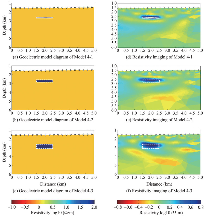Figure  14  Electrical resistivity imaging of vertically dispersed models of various lengths in offshore CO₂ storage for Models 4-1, 4-2, and 4-3

Download: Full-Size Img

Figures 14(a)‒(c) are schematic diagrams of Models 4-1, 4-2, and 4-3, respectively. Dark blue represents the range of offshore CO₂ diffusion areas, light yellow represents marine sediments, and white boxes represent offshore CO₂ reservoirs. Figures 14(d) ‒ (f) are resistivity imaging for Models 4-1, 4-2, and 4-3, respectively.

The length of the high-resistivity area basically corresponds to the length range of the offshore CO₂ storage. However, there are significant differences in the inversion results of offshore CO₂ (Models 4-1, 4-2, and 4-3) with different longitudinal dispersion ranges. In Model 4-1, the inversion depth and regional range of the top of the offshore CO₂ storage are closest to the simulated depth and regional range. In comparison, in Models 4-2 and 4-3, the inversion depth and regional range of the offshore CO₂ storage gradually deviate from the simulated model as the vertical dispersion range of offshore CO₂ gradually decreases. However, the approximate range of the model can still be obtained to determine the approximate position of the target body.

For the inversion of Model 4, the curve of RMS misfit and roughness change with the number of iterations is shown in Figure 15.

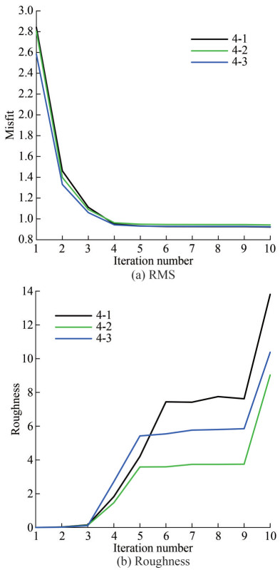Figure  15  RMS and roughness curve inversion with iterations of Models 4-1, 4-2, and 4-3, respectively (Black, green, blue)

Download: Full-Size Img

As shown in Figure 15, roughness increases with the increase of iterations. In addition, the RMS misfit of Occam inversion converges with the increase of iterations, and the target misfit is 1. The inversion RMS misfit of the four models all reach the target misfit in the 7th iteration, thus proving that the inversion results are reliable. The comparison between model inversion data and actual target data is shown in Figure 16.

Figure  16  Amplitude and phase of data and inversion of the E_y electric field response vs. transmitter position for Model 4-1

Download: Full-Size Img

The curves from top to bottom correspond to Models 4-1, 4-2, and 4-3 respectively (Figure 16). By comparing the error ranges of the inversion target bodies of different models at two frequencies of 0.25 Hz (blue curve) and 0.75 Hz (green curve), we find that the difference between the resistivity inversion values and the real values is relatively small. This means that the observed error of the inversion effect is relatively stable for target bodies of different thicknesses. The inversion results of the three models have little difference from the actual target bodies.

3.6   Various adjacent saturation models

The effects of the resistivity imaging of two offshore CO₂ saturation models (Models 5-1 and 5-2) for offshore CO₂ models are shown in Figure 17(c)(d), respectively. The high-resistivity range and high saturation range obtained by imaging are consistent with the reservoir range of the model. Several common offshore CO₂ adjacent saturation types that need to be compared in this group of models are shown in Table 7.

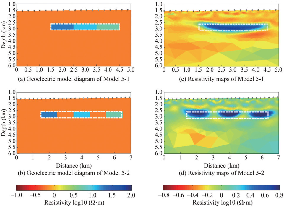Figure  17  Electrical resistivity imaging of lateral migration at various intervals in the offshore CO₂ storage for Models 5-1 and 5-2

Download: Full-Size Img

Figures 17(a) and (b) are schematic diagrams of Models 5-1 and 5-2, with dark blue color indicating the extent of offshore CO₂ dispersion area, light yellow color indicating marine sediment, and white box indicating offshore CO₂ reservoir; Figures 17(c) and (d) are resistivity maps of Models 5-1 and 5-2.

The depth of the high-resistivity area basically corresponds to the depth range of the offshore CO₂ reservoir. However, the inversion results of the two models are still different. In particular, the inversion depth and regional area range of adjacent offshore CO₂ reservoirs with different saturation in Model 5-1 are the closest to the depth and regional range of the model simulation target. In comparison, in Model 5-2, the adjacent distance of the target body with different saturation becomes wider, and the inverse resistivity imaging image can still clearly reflect the burial depth, regional range, and boundary of each simulated target body, thus resulting in high-quality resistivity imaging. For the inversion of model 5, the curve of RMS misfit and roughness change with the number of iterations is shown in Figure 18.

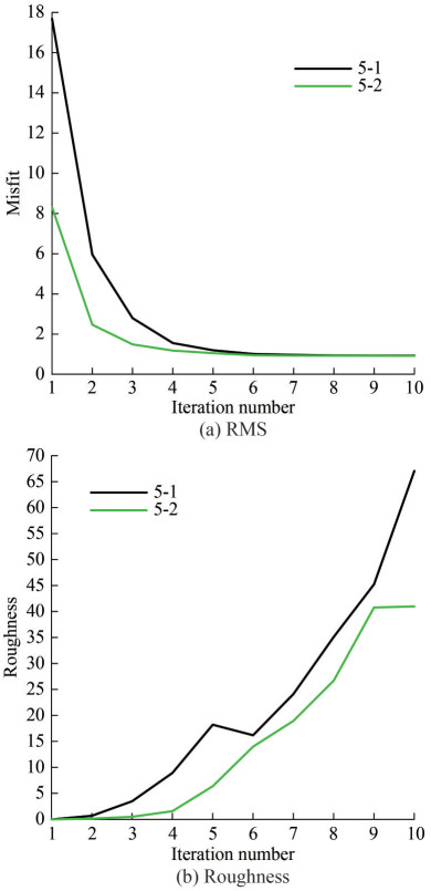Figure  18  RMS and roughness curve inversion with iterations of Models 5-1 and 5-2, respectively (Black, green)

Download: Full-Size Img

As shown in Figure 18, roughness increases with the increase of iterations. In addition, the RMS misfit of Occam inversion converges with the increase of iterations, and the target misfit is 1. The inversion RMS misfit of all four models can reach the target misfit in the 7th iteration, thus proving that the inversion results are reliable. The comparison between model inversion data and actual target data is shown in Figure 19.

Figure  19  Amplitude and phase of data and inversion of the E_y electric field response vs. transmitter position for Model 5-1

Download: Full-Size Img

The curves from top to bottom correspond to Models 5-1 and 5-2, respectively (Figure 19). Upon comparing the error ranges of inversion target bodies of different models at two frequencies of 0.25 Hz (blue curve) and 0.75 Hz (green curve), we find differences between the inverse value of resistance and the real value, although the inversion results of the two models are not very different from the actual target bodies, and the error ranges are relatively stable.

4   DCharacteristics and influencing factors

4.1   Influence of operating conditions

A previous study (Yilo et al., 2023) has reported that CSEM performs well in monitoring vertical leakage and providing comprehensive assessments compared with seismic methods. In contrast, our work pays more attention to the transverse transport resolution of CO₂. In this work, five common migration situations were divided into the establishment of the migration model, and inversion simulation and iterative misfit analysis were carried out, thus providing a more comprehensive reference for the monitoring role of CSEM in the entire CO₂ storage work. Furthermore, by tracking the migration situation, CO₂ reserves could be estimated in advance, and potential leakage risks could be assessed. We also discussed the impact of the following four factors on the monitoring results.

1) Influence of offset on monitoring. When the offset is less than 3 km, the electric field characteristic curves of each model almost coincide, and the observation system basically has no response to the target. When the offset exceeds 3 km, the electric field signals collected by the observation system to monitor the CO₂ plume begin to separate from the background. Therefore, if we want to observe more obvious signal characteristics, we should select the offset of 6–7 km, in which the electric field response characteristics at each frequency are the most obvious.

2) Influence of burial depth on monitoring response. Based on the inverse resistivity image in Figure 7, when the burial depth of the CO₂ reservoir is 2 km, CSEM's monitoring and inversion results have begun to deviate from the actual target. This finding indicates the weak reflected signal at this depth and the lost discernability of its response amplitude. Therefore, the shallower the burial depth, the better the response characteristics obtained by CSEM monitoring. Thus, it is necessary to transmit higher power signals to identify the buried high-resistance anomalous body.

3) Influence of frequency on monitoring. By comparing the response characteristics of each electric field component at five different frequencies, the offset corresponding to the inflection point of the electric field response curve at different frequencies tends to vary. The higher the frequency, the smaller the offset required for the abnormal electric field response to reach the peak value, and with the increase of the offset, the stronger the influence of the airwave. Therefore, in the CSEM monitoring work, on the premise of achieving the detection target, asmaller frequency selected translates to reduced interference. For example, 0.25 Hz in the experiment has the best electric field response under each component compared with other higher frequencies.

4) Influence of different components on monitoring. As shown in Figures 3 ‒ 4, the responses of various frequencies under the three electric field components are compared. Compared with other components, the electric field response characteristics obtained by the E_y component under each frequency measurement are more stable and demonstrate more regular changes. Therefore, E_y has a more stable monitoring capability in terms of lateral resolution.

4.2   Influence of monitoring time

The influence of monitoring time on the results mainly comes from the influence of the change in CO₂ migration distance; thus, the length of the source and receiver must be changed. Furthermore, the longer the monitoring time, the larger the offset that needs to be laid.

4.3   The influence of uncertainty

The inversion algorithm affects the resolution of inversion results, and different inversion parameters may lead to varying inversion results. Therefore, to obtain better inversion results, more parameters must be tested.

4.4   Comparison between the seismic and electromagnetic methods

The seismic method is considered a costly and cost-effective technique that can provide high-resolution images of structures and formations. However, in many cases, the seismic method alone is not sufficient to distinguish between fluids and their saturation. Compared to the seismic method, CSEM is a low-cost CO₂ monitoring technique; its resistivity has a clear response to changes in fluid type and saturation, and it can be used to estimate CO₂ saturation (Fawad and Mondol, 2021).

5   Conclusions

1) This study investigates the sensitivity of the ocean CSEM in monitoring plume transport during offshore CO₂ storage. Through simulation experiments and data analysis, we found that this method can effectively detect and monitor the transport path and velocity of CO₂ in the ocean.

2) This study not only provides a reference for the study of offshore CO₂ sequestration plume migration mechanism but also proposes a method and provides technical support for CO₂ sequestration monitoring.

3) In future studies, the experimental model can be further optimized; multiple influencing factors, such as emission source frequency, can be integrated; and joint application with other geophysical methods can be explored to improve the accuracy of monitoring work.