1   Introduction

Subsurface rockophysical modeling and time-lapse seismic monitoring are two key technologies in CO₂ storage. The former can establish the bridge between elastic and reservoir parameters by simulating the actual situation of the seabed formation; the latter is to obtain the changes of subsurface velocity, density, impedance and other parameters through inversion, so as to evaluate the location and state of CO₂. Most CO₂ sequestration projects worldwide involve rockophysics and time-lapse seismic monitoring. Among them, several famous projects include the Weyburn-Midale project in Canada (IEA GHG Weyburn-Midale CO₂ Monitoring and Storage project) (White, 2009, 2013; Smith et al., 2018), the In Salah project of BP in Algeria, the Aquistore project of Saskatchewan Power Plant and Petroleum Technology Research Centre in Canada, and the Ketzin Project of the European Union in Germany. In terms of offshore CO₂ storage, the famous projects that have been in operation are the Sleipner and Snovit project in Norway, and the Tomakomai project in Japan. In Europe, there are several offshore carbon storage projects centered in the North Sea. In the future, the Northern Lights in Norway and Greensand in Denmark, are expected to be active in 2024 and 2025, respectively (Patil et al., 2023).

Although rockphysical modeling and time-lapse seismic monitoring have been successful operated in many domestic and international CO₂ sequestration projects (Alfi and Hosseini, 2016; Wang et al., 2017), the case has not been applied to offshore carbon sequestration in China. The temperature and pressure conditions in the shallow seabed formation, the seismic data acquisition is different from land condition. And there are also many differences in implementation and expense. At present, there is a lack of expense research and understanding of whether CO₂ offshore sequestration can be carried out with better time-lapse seismic monitoring effects and the physical significance of the differences in time-lapse seismic monitoring. After the current small-scale experimental CO₂ injection in the South China Sea in China, the simulation study of its geology environment and the forward analysis of time-lapse seismic monitoring, especially the effect of formation pressure on seismic data, need to be further studied.

The establishment of a time-lapse seismic forward model is the basis of seismic inversion. The main factor for accurate calculation of seismic forward modeling is the elastic parameters during CO₂ injection. Especially the P-wave and S-wave velocity and density. Because they are the most prominent parameters affecting the time-lapse seismic forward modeling. During the CO₂ injection process, the reservoir pressure as well as fluid saturation changed, which affected the P-wave and S-wave velocity and density. In the offshore, the cost of drilling and logging is very high. Furthermore, the reservoir information acquired by logging methods is very limited. Therefore, the detailed rockphysical model is necessary to simulate the reservoir. Then, with the help of anisotropic exact reflection coefficient equation, the more accurate forward can be obtained (Ma and Morozov, 2010).

In the situation that no events of fracturing, collapse, and subsidence before and after CO₂ injection, the difference in amplitude and travel time between the two seismic monitoring mainly comes from the effect of fluid saturation and formation pressure (Li et al., 2017). This condition is the result of reservoir elastic parameters varied by saturation and pressure. Understanding the changing trend of elastic parameters with formation pressure and CO₂ saturation is important to time-lapse seismic forward modeling. Another way to obtaining this relationship is cores analyzing. It can get a statistical relationship. However, such statistical results are limited by the quantity and location of cores. And this method lacks the support of rockphysical theories (Wang et al., 2019, Wang et al., 2022). This lead to a poor generalization. Therefore, it is very necessary to establish a more reasonable and comprehensive research method based on rockphysical theory (Wang et al., 2020).

Specifically, in conjunction with the actual seafloor formation geological situation, a rockphysical model that can take into account varieties of influencing factors (mineral composition, pore aspect ratio, fracture, fluid distribution, formation pressure, and anisotropy) is proposed. Through the rockphysical model, the change of P-wave and S-wave velocity during CO₂ injection can be obtained. Then the reflection coefficient is calculated by the anisotropic exact reflection coefficient equation. With the reflection coefficients, together with the commonly used Ricker wavelet, the seismic record is calculated by the convolution model. In this way, the relationship between formation pressure (and CO₂ saturation) and seismic record is established. This contributes to analyzing the influence of formation pressure and CO₂ saturation on the time-lapse amplitude versus offset (AVO) interpretation during the CO₂ injection process. The conclusion provides a theoretical basis for the time-lapse seismic interpretation and monitoring.

2   Rockphysics modeling

2.1   Equivalent elastic modulus of VTI background medium

For rocks with complex mineral compositions, the equivalent medium theory can be used to calculate the modulus of mixed minerals. Compared with the frequently used Voigt-Reuss boundary and Hill's average, the upper and lower bounds of the Hashin Shtrikman boundary (Hashin and Shtrikman, 1962, 1963) are the narrowest allowable upper and lower bounds (Mavko et al., 2020). Therefore, the arithmetic average value of Hashin-Shtrikman boundary is used as the equivalent modulus of mixed minerals. The original Hashin-Shtrikman boundary is suitable for two components. Berryman (1995) deduced a more general form of Hashin-Shtrikman boundary for calculating more than two components:

where,

K^HS+ and K^HS− are the upper and lower bounds of bulk modulus, μ^HS+ and μ^HS− are the upper and lower bounds of shear modulus, K(r) and μ(r) are bulk modulus and shear modulus of each component. The braces indicate the average of materials, that is, the weighted average of each component according to its volume content.

The Hertz-Mindlin contact theory is to equate the rock as an accumulation of some same-sized grains, by calculating the positive and tangential stiffnesses between two grains under certain external forces, and then obtaining the equivalent modulus of an arbitrary equal-size accumulation of grains (Mindlin, 1949). On the basis of the Hertz-Mindlin contact theory, many scholars have made different aspect improvements to this theory (Walton, 1987; Digby, 1981; Jenkins et al., 2005; Norris and Johnson, 1997; Dvorkin and Nur, 1996). Among them, Dvorkin improved the model by taking into account the sorting of the grains inside the rock. In this way, though considering the relaxation between grains and the irregularity of the contact surface among grains, it is possible to simulate the characteristics of the actual seafloor formation. Especially the weak consolidation and variation of grains sizes, etc. The expression of Dvorkin's improvement can be summarized in the following form.

where, ν is the Poisson's ratio of mineral, R is the curvature radius of the contact surface, f is non-smooth contact percentage, R is the effective contact radius, P is the effective pressure at the point of grains contact. The deduction in Hertz-Mindlin theory involves the Hashin-Shtrikman boundary model(Hashin and Shtrikman, 1962, 1963). The equation can be used to calculate the bulk and shear modulus at a given depth by assuming mineral composition, porosity, and overburden stress. As shown in equations (3) and (4), unless the granular aggregates are composed of the same spherical grains (R/R=1), the calibration parameter are dependent on the coordination number n and ratio R/R. R/R can be greater than or less than 1. The ratio takes into account the smoothness and sorting of grains, and can be regarded as a parameter that characterizes the average effective contact radius and general grains size distribution.

After obtaining the modulus of various mineral mixtures, the stiffness coefficient of the VTI background medium can be calculated. The elastic parameters of anisotropic thin layered strata composed of multiple isotropic layers are calculated by Backus average (Backus, 1962). Although the assumption of Backus average is long wavelength, for horizontally layered anisotropic medium, the usage on the logging scale is effective (Hsu et al., 1988; Imhof, 2003; Liner, 2006). The VTI equivalent medium by Backus average can be written as the stiffness matrix,

where, the relationship between stiffness coefficient and elastic parameters of each layer is as follows:

where superscript B represents the calculation result of Backus average, λ and μ are Lamé coefficient.

2.2   Equivalent elastic modulus of dry rock skeleton with pores

In the seafloor, the porosity is relative high. The effective medium theory can be used for simulation this condition. Hornby et al. (1994) studied the effective elastic properties by using the effective medium model. The model combines anisotropic self-consistent approximations model (SCA) with anisotropic differential effective medium model (DEM). Many scholars (Yuan, 2007; Qian, 2017; Zhao, 2017) have obtained two perceptions after forward simulation calculations. One is that the anisotropic SCA can ensure that the matrix and fluid of rock are connected in two-phases only when the porosity is within 40%‒60%. Therefore, for the solid – liquid two-phase mixture, to simulate the actual two-phase connection rock structure, the anisotropic SCA model is used to calculate the equivalent stiffness tensor when the fluid content is 50%, and then the anisotropic DEM model is used to adjust to the specific porosity to obtain the calculation results of anisotropic SCA+DEM. The other is a disadvantage of DEM. The DEM formulation does not treat each constituent symmetrically. There is a preferred matrix or host material, and the effective moduli depend on the construction path taken to reach the final composite.

For multiple inclusion shapes or multiple constituents, the effective moduli depend not only on the final volume fractions of the constituents but also on the order in which the incremental additions are made. The anisotropic SCA+ DEM model can be written as.

where, c represents the calculated equivalent medium stiffness tensor; v is the volume content of the inclusion; cⁱ is the stiffness tensor of the inclusion; The tensor $\stackrel{\wedge}{G}$ is Eshelby tensor (Eshelby, 1957), which controls the shape of pores, and its expression contains the aspect ratio. The derivation and calculation process of $\stackrel{\wedge}{G}$ are given in the form of line integral (Kinoshita and Mura, 1971; Mura, 1991).

2.3   Equivalent elastic modulus of dry rock skeleton with fractures

Overpressure fluids and gases can cause the formation of fractures in muddy sediments (Sassen et al. 2001). Figure 1 shows a fracture filled natural gas hydrate model, Using the linear slip theory, the VTI background medium is embedded with horizontal direction parallel fractures (Hsu et al. 1988; Sondergeld and Rai, 2011). With the help of this step, the rockphysical model considers both the anisotropy caused by the directional arrangement of minerals and fractures. This is more relevant to the reality of the underground situation. The assumptions of the model are consistent with Schoenberg and Helbig's model, ignoring the influence relationship between horizontal and vertical symmetry. The elastic coefficient matrix form of the above theory can be written as follows:

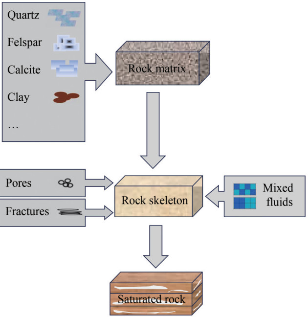Figure  1  The rockphysics model schematic workflow

Download: Full-Size Img

where subscript b represents the stiffness coefficient of VTI background matrix. Combining Schoenberg and Helbig's theory with Hudson's theory (Hudson, 1980, 1981), the expressions of normal weakness ΔN and tangential weakness ΔT can be obtained based on linear anisotropy approximation.

where, g = V_S²/V_P², ε^V and δ^V are two of anisotropic parameters proposed by Rüger (1997) on the analogy with Thomsen VTI anisotropic coefficients (Thomsen, 1986):

2.4   Calculation of mixed fluid modulus and fluid substitution

For saturated rocks with two or more fluids, the equivalent bulk modulus of the mixed fluids is required for fluid replacement. The earliest theory on fluid mixing modulus was proposed by Wood and Hill as the upper and lower limits (Wood, 1955; Hill, 1963). For the case of gas-water saturation, Brie et al. (1995) proposed an equivalent bulk modulus empirical equation. The above is calculating the mixed fluid modulus from the perspective of fluid distribution. From the aspect of rock microstructural description, harmonic and arithmetic averaging at the endpoints and capillary pressure in pores, the mixed fluid modulus is described as (Papageorgiou et al., 2016):

This equation has a solid theoretical foundation. The theory exactly produces both a serial and a parallel law. For the limiting values of the capillary pressure coefficient parameter α, equation (11) reduces analytically to harmonic (α = K_w/K_g) or arithmetic (α = 1) averaging at the endpoints.

The Brown-Korringa theory (Brown and Korringa, 1975) describes the relationship between the effective elastic tensor of anisotropic dry rock and fluid-saturated rock. It is commonly regarded as the improved anisotropic Gassmann model. Its equation can be expressed as equation (12).

where S_ijkl^dry, S_ijkl^sat, and S_ijαα⁰ represent the effective elastic compliance of dry rock, fluid saturated rock and solid minerals respectively. β_fl = 1/K_fl and β₀ = S_aαββ⁰ = 1/K₀ represent the fluid and mineral compressibility respectively. ϕ is rock porosity.

At last but not least, the vertical direction P-wave velocity and S-wave can be calculated by:

The flow chart of the rockphysical modeling process is shown in Figure 1 and Figure 2.

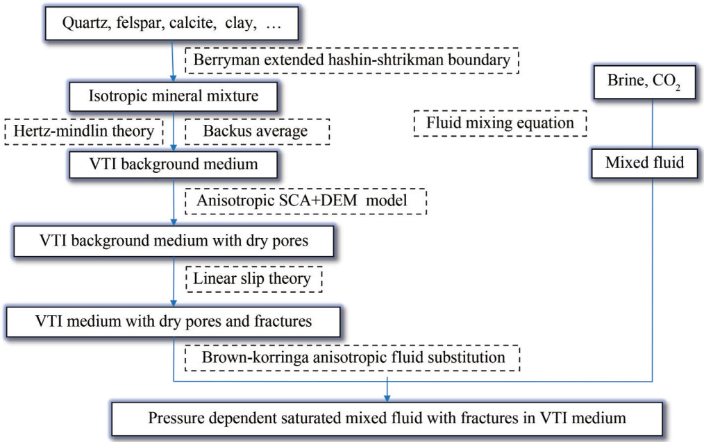Figure  2  The flow chart of rockphysical modeling for calculation of elastic tensor

Download: Full-Size Img

3   The effect of formation pressure, porosity and CO₂ saturation on velocity

From the rockphysical model proposed above, the effect of formation pressure, porosity and CO₂ saturation on the velocity can be obtained by inputting information and data from welling, logging, and cores in an area in the South China Sea.

The actual data comes from the Pearl River Estuary Basin. The Pearl River Estuary Basin is a Cenozoic continental margin extensional basin formed on the Tertiary basement, and is also a major oil and gas producing area in South China Sea. The specific location is on the west side of the depression. This region is rich in material sources and has a complex and diverse composition of minerals. Multiple wells have produced oil and gas flows since 2016, revealing the enormous exploration potential of the region. Due to multiple factors such as sedimentary environment, diagenesis, secondary transformation of oil and gas migration, and engineering drilling, this area currently has the following characteristics: shallow burial (1 000‒1 400 m), thin interbed layers (1‒4 m), fine layer grains (argillaceous siltstone, thin interbedded siltstone), and locally developed horizontal fractures. These features are consistent with the characteristics of proposed rockphysical model.

The parameters of target layer are shown in the table, which are the input for rockphysical forward modeling.

The first is the effect of formation pressure on the velocity. Because the injected CO₂ pressure is greater than the formation pressure, the CO₂ injection will definitely affect the formation pressure, which in turn changing the P-wave and S-wave velocity. In Figure 3, the formation pressure is positively correlated with the velocity. Analyzed from the geological point of view, the increase of formation pressure mainly increases the degree of compaction of rock skeleton and increases the modulus, which in turn makes the velocity increase. This can also lead to pore pressure increasing. Especially existing the overlying gap layer, the fluid space is relatively limited, and the increase in pore pressure may be more pronounced. Moreover, the elastic parameters in supercritical state CO₂ vary more with pressure than in seawater.

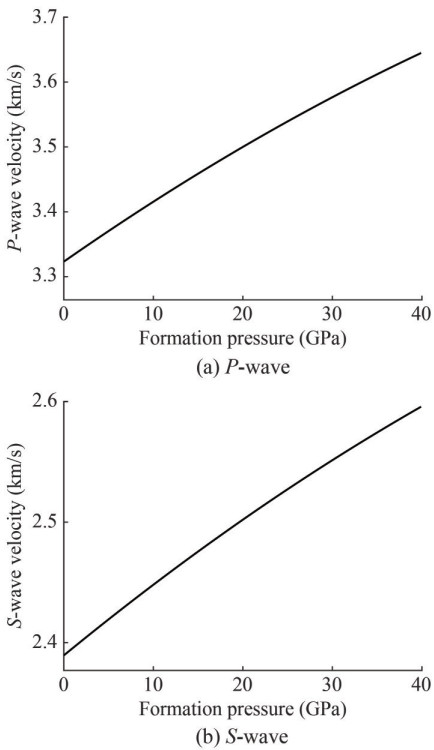Figure  3  The influence of formation pressure variation on P-wave and S-wave velocity

Download: Full-Size Img

The effect of porosity on velocity can also be concluded from the rockphysical model. In Figure 4, it can be seen that the porosity is negatively related to the velocity. One of the main reasons for this is that the formation become harder, denser, modulus getting bigger, which can cause velocity increasing. In addition, after CO₂ injection, under suitable temperature and pressure conditions, CO₂ hydrate may be generated within the formation, resulting in porosity decreasing, which will also lead to the velocity increasing.

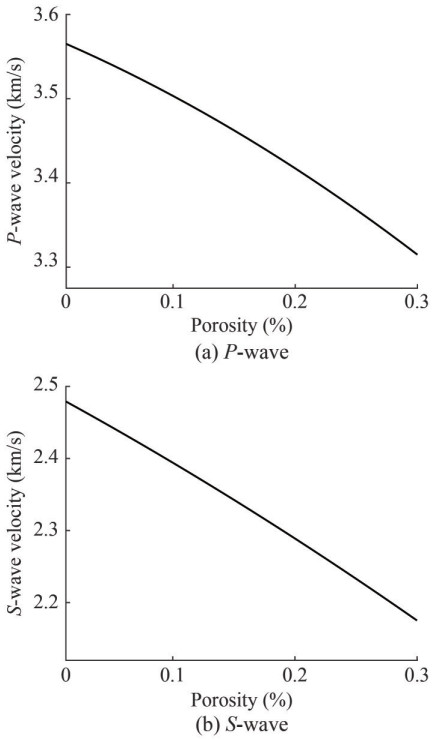Figure  4  The influence of porosity variation on P-wave and S-wave velocity

Download: Full-Size Img

The last important influence on CO₂ sequestration is the saturation of CO₂. In Figure 5, as CO₂ injected, the saturation of CO₂ becomes higher, the saturation of seawater becomes lower, the P-wave velocity decreases, and the S-wave velocity remains essentially unchanged. The S-wave velocity is mainly affected by the solid medium, so the change of the type and amount of fluid in the formation pore space has almost no effect on the S-wave. Relatively, the impact of CO₂ saturation on velocity is not as significant as the impact of formation pressure on velocity. It is a bit difficult to detect saturation using seismic methods.

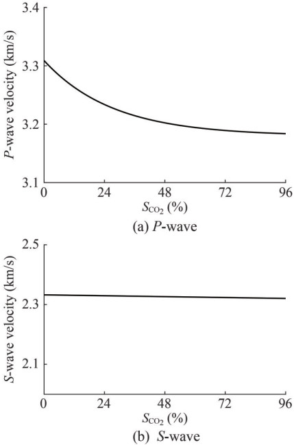Figure  5  The influence of CO₂ saturation variation on P-wave and S-wave velocity

Download: Full-Size Img

Through the forward analysis of the rockphysical model above, the formation pressure has the greatest impact on velocity, followed by porosity and CO₂ saturation. Thus, the formation pressure has a significant impact on the elastic properties of relatively loose seabed formation.

4   The effect of formation pressure, porosity and CO₂ saturation on reflection coefficient

Formation pressure, porosity and CO₂ saturation have an effect on the velocity, so these two parameters certainly have an effect on the reflection coefficient. Based on the anisotropic exact reflection coefficient equation (Wu et al., 2022), it is possible to simulate the seafloor formation and obtain the variation of the reflection coefficient. This reflection coefficient equation corresponds to the rockphysical model proposed above, applicable to anisotropic formation. The equation is not a linear approximate equation and have high computational accuracy.

As shown in Figure 6, varieties of formation pressure, porosity, and CO₂ saturation cause different reflection coefficient. The changing of reflection coefficient caused by formation pressure is the most pronounced, especially for big incidence angle. Porosity also has an effect on the reflection coefficient. The bigger the porosity, the smaller the reflection coefficient. This is in accordance with general geologic knowledge. For the effect of CO₂ saturation on reflection coefficient, as mentioned above in the manuscript, changes in the CO₂ content in the pore and fracture space do not affect the S-wave velocity and have little effect on the P-wave velocity. There is also little difference in density between supercritical CO₂ and seawater. This gives rise to the fact that changes in the CO₂ saturation have almost no effect on the reflection coefficient. That is, the reflection coefficient basically only varies with incidence angle (known as the AVO effect), as shown in Figure 6(c).

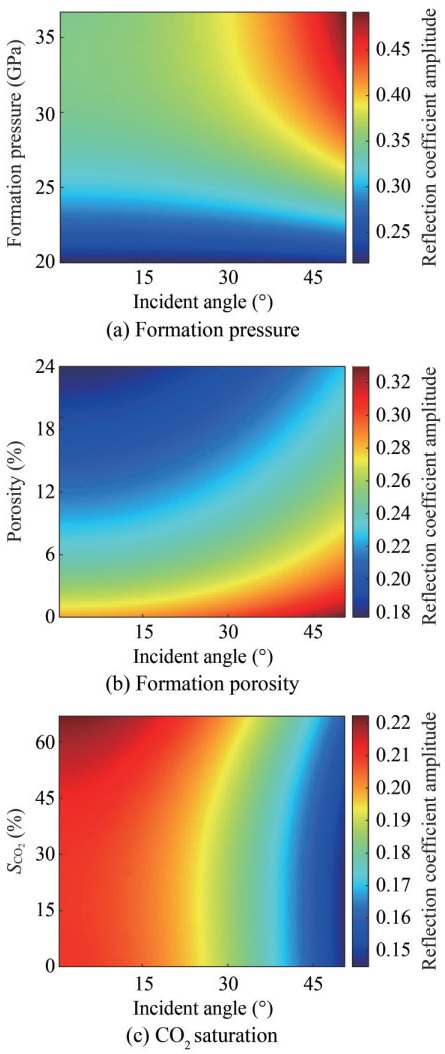Figure  6  The influence of formation pressure, porosity, and CO₂ saturation variation on reflection coefficient amplitude

Download: Full-Size Img

5   The effect of formation pressure, porosity and CO₂ saturation on seismic record

AVO method is used to study the seismic reflection amplitude variation characteristics between the shot point and the receiver the shot offset, and then detect the underlying media information at the reflection interface. AVO is currently the most important and commonly used method for reservoir exploration.

The VTI media exact reflection coefficient equation has no assumptions of small incident angle and weak impedance differences. So it is more applicable and computational accuracy (Wu et al. 2022). The specific form of the equation can be found in Appendix. Then using convolutional model, VTI media seismic records are obtained from the calculated reflection coefficients. In the calculation, we use the commonly used Ricker wavelet with a main frequency of 30Hz. The incidence angle is 6°‒ 26°, with an interval of 3°.

During the CO₂ injection stage, most logging methods cannot be used due to the influence of casing in the well. Moreover, the CO₂ saturation and formation pressure changed simultaneously. Here, reservoir pressure data is obtained through pressure sensors on the wellbore at the perforation location. The saturation of CO₂ in the reservoir can be roughly calculated based on parameters such as the cumulative injection of CO₂, reservoir capacity, and porosity. In summary, through calculation, during the process of CO₂ saturation ranging from 20% to 60%, the formation pressure increased from 1.2 MPa to 1.6 MPa. The seismic records performed before and after this process are shown in Figures 7(a) ‒ (b). And the difference between the two seismic records is shown in Figure 7(c). Figure 7(c) illustrate the difference in seismic records mainly occur in far offset and large wave impedance differences areas. This is because formation pressure has a greater impact on velocity changes at large offset distance (incidence angle). And big wave impedance differences in this area could increase this impact. The target layer is located near 0.51 s two-way travel time. In Figure 7(b), the AVO characteristic presents a strong negative polarity amplitude with zero offset and have an increasing trend. This layer has a lower wave impedance than the overlying medium. This characteristic is very similar to the class Ⅲ AVO characteristic. Class Ⅲ AVO characteristic manifested as a poorly compacted or unconsolidated low impedance gas bearing sandstones reservoir characteristic (Ismail et al., 2020). This also indicates that the seismic response of supercritical CO₂ is similar to natural gas. Fortunately, the class Ⅲ AVO characteristic can easily detected in shallow seabed formations by conventional seismic techniques.

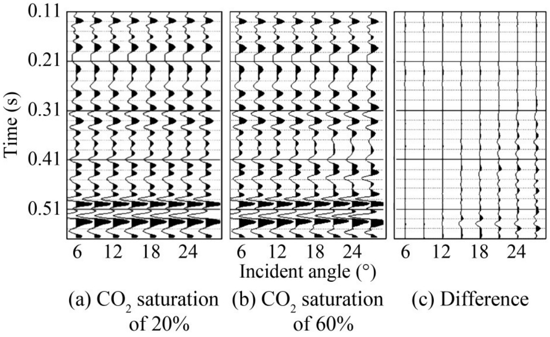Figure  7  Seismic records forward modeling results with CO₂ saturation of 20% (a) and 60% (b) and their difference (c)

Download: Full-Size Img

6   Conclusions

The construction difficulty, period and cost of offshore seismic surveys are much larger than onshore condition. Currently, there are many successful cases of onshore carbon sequestration projects in China. However, the domestic offshore carbon sequestration project has just been carried out, so applying offshore seismic survey to image the CO₂ sequestration reservoir requires lots of work. Here, a rockphysical model that takes into account the various minerals composition of rock matrix and various fluids composition, fracture, fluid distribution, and anisotropy is proposed for the seabed carbon sequestration area. The submarine formation is simulated in sufficient detail and determine the relationship between the elastic and reservoir parameters. After that, the reflection coefficient is calculated from the anisotropic exact reflection coefficient equation, and the seismic record is obtained from the convolution model. After the above steps, it is possible to forward modeling the effect of reservoir parameters (especially pressure, the main parameter affecting the phase state of CO₂ in shallow submarine formation) on the seismic record. The three forward modeling (physical parameters on velocity, reflection coefficients and seismic records) lead to the following insights:

1) Rockphysical modeling for the target layer is the foundation of time-lapse seismic monitoring. The establishment of a rockphysical model can simulate submarine geological characteristics in detail and introduce reservoir parameters in seismic domain.

2) After filling CO₂ into the pore and fracture, the formation pressure has a greater effect on the velocity, reflection coefficient, and seismic record. Specifically, it brings about the velocity and reflection coefficients increasing.

3) After injecting CO₂ into the formation, the "bright spot" that similar to the Class Ⅲ AVO characteristic in unconsolidated formation may be shown in the seismic record. This indicates that it is possible to carry out time-lapse seismic monitoring at different CO₂ marine geological storage stages.

Appendix An exact reflection coefficient equation for VTI media

The Thomsen anisotropy parameters (Thomsen, 1986) mainly describe the relationship between two vertical velocities, three dimensionless anisotropy parameters and five stiffness coefficients based on the weak anisotropy assumption. The relations are as follows:

where V_P and V_S denote the P- and S- wave velocity in the vertical direction (symmetry axis direction) respectively, ρ denotes the density, and ε, δ, and γ are the Thomsen anisotropy parameters. Since the SH-wave is completely decoupled from the P- and SV- waves in VTI media, the reflection and transmission coefficients of the P- and SV- waves are considered.

Based on the weak anisotropy assumption, the P-wave phase velocity and stiffness coefficient c₁₃ in the VTI media can be linearly expressed by anisotropy parameters ε and δ as (Thomsen, 1986).

According to Equation (A2), a relatively simple form of horizontal slowness (ray parameter) can be obtained.

Substituting Equation (A1) and (A3) into the VTI media exact reflection coefficient equation (Graebner, 1992; Schoenberg and Protázio, 1992; Rüger, 1996). Then the following matrix can be obtained:

Like exact Zoeppritz equation (Zoeppritz, 1919; Aki and Richards, 1980), equation (A5) can be expressed in the following equation:

In Equation (A5), the coefficients of the matrix are given by,

The superscripts ⁽¹⁾ and ⁽²⁾ indicate the upper and lower layer respectively,

where,

In the above equations for the VTI reflection and transmission coefficients, the vertical slowness of the different wave modes can be expressed as (Rüger, 1996):

where,

and q_α is the vertical slowness of the P-wave, q_β is the vertical slowness of the SV-wave, c_ij is the stiffness tensor, and θ is the phase angle. The subscript α and β denote the P-wave mode and SV-wave mode respectively.

Substituting Equations (A1) and (A2) into Equation (A10), replaced the independent stiffness coefficients by the Thomsen anisotropy parameters.

Equation (A5) is an implicit equation of the VTI media reflection and transmission coefficients. Equations (A4), (A7), (A8), and (A9) are the intermediate variables of Equation (A5).