1   Introduction

Offshore carbon capture, utilization, and storage (OCCUS) is an important technology for greenhouse gas mitigation (Vandeweijer et al., 2011; Hansen et al., 2013; Furre et al., 2017; Ringrose and Meckel, 2019; Flohr et al., 2021; Roche et al., 2021). CO₂ mitigation can be realized through OCCUS technology, which is a solution and technological system developed by coastal countries or regions through engineering methods. Compared to onshore CO₂ storage technology, OCCUS technology offers several advantages, such as extensive storage sinks and enhanced security (Meckel et al., 2017; Eide et al., 2019; Suicmez, 2019; Li, 2022). CO₂ injection changes the elastic parameters of the subsurface media, and therefore the seismic response. This makes seismic methods are crucial tools for monitoring CO₂ injection. Seismic methods offer the potential to collect com-prehensive data on elastic parameters and reservoir properties, including lithologies, porosity, and the state of pore fluids. These data can supply detailed information that is valuable for understanding the subsurface environment during CO₂ injection (Bosch et al., 2010). Seismic methods have been extensively applied in various CO₂ storage projects during the past two decades to monitor the migration of subsurface CO₂ plume (Arts et al., 2004; Daley et al., 2007; Saito et al., 2008; Harris et al., 2016; Wang and Morozov, 2020; Li et al., 2023). The migration of CO₂ plume is successfully identified through migrated images, velocity differences, or reservoir parameters using these applications.

With the advancement of OCCUS, a recognized need for the quantitative estimation of CO₂ and detailed monitoring of its flow path emerges. Among various seismic methods available, full-waveform inversion (FWI) is continuously gaining increasing attention due to its potential to realize the highest resolution (Tarantola, 1984; Virieux and Operto, 2009; Zhang et al., 2019). Recent studies (Queißer and Singh, 2013; Li et al., 2021; Hu et al., 2023) have shown that time-lapse FWI of repeated seismic surveys can accurately estimate high-resolution variations related to CO₂ injection. A direct relationship is observed between these parameters and the reservoir properties of the CO₂ storage site. Thus, time-lapse FWI is considered a valuable tool for quantitative analysis and monitoring of CO₂ flow in underground storage sites. Regardless of its success, FWI encounters challenges in practical OCCUS projects due to the cycle-skipping problem associated with the conventional point-to-point minus-type objective function. The accuracy and efficiency of the inversion process can be restricted by this issue (Tarantola, 1984; Virieux and Operto, 2009). Furthermore, the difficulties encountered by FWI in practical OCCUS projects are further exacerbated by practical issues, such as limited aperture, absence of low-frequency data, unknown seismic wavelets, and inaccurate initial models (Virieux and Operto, 2009).

Researchers have introduced different variants of FWI to address the challenges associated with the conventional approach (Bunks et al., 1995; Sirgue and Pratt, 2004; Djebbi and Alkhalifah, 2014; Métivier et al., 2018). One basic idea involves using portions or subsets of the full information contained in seismic data. For instance, the frequency continuation strategy can mitigate the cycle-skipping problem by using the low-frequency data firstly and feed in the high-frequency data successively (Bunks et al., 1995). Travel time is an important piece of information that supports seismic data analysis. This information represents the time taken for seismic waves to propagate from the sources to the receivers. The incorporation of travel-time information into the FWI frame facilitates the inversion of the elastic parameters, which are called skeletonized FWI or travel-time-based FWI in the literature (Luo and Schuster, 1991; Tromp et al., 2005; Ma and Hale, 2013; Lu et al., 2017). Travel-time-based FWI is extensively applied in geoscience applications due to the quasilinear behavior of its objective function and reduced sensitivity to noise (Dahlen et al., 2000; Montelli et al., 2004; Pyun et al., 2005).

An essential component of travel-time-based FWI is the determination of travel-time shifts between the simulated seismic signals and the observed seismic signals collected before/after the injection. The travel-time shifts expose the disparity between the compared signals, with larger shifts indicating greater differences between the current baseline/initial models and the postinjection models. Cross-correlation and dynamic time warping (DTW) are two commonly used methods for travel-time shift estimation (Knapp and Carter, 1976; Hale, 2013). The small shift limitation of cross-correlation and the instability and high sensitivity to noise of DTW seriously plague their applications in complex situations (Wang et al., 2023). Cross-correlation-based dynamic time warping (CDTW) is a leading technique for estimating travel-time shifts. The CDTW method combines the benefits of the commonly used cross-correlation and DTW methods (Wang et al., 2023), enabling automatic estimation of time-varying shifts with robustness.

A novel time-lapse FWI method, in which CDTW is used to measure the discrepancy between simulated and observed seismic signals of baseline and monitor seismic data, is developed in the current study. The abbreviation time-lapse CDTW-FWI is adopted for the proposed method to enhance clarity. In the CDTW-FWI method, the objective function is constructed using the L2 norm of the travel-time shifts estimated by CDTW. Limited-memory Broyden–Fletcher– Goldfarb–Shanno (LBFGS) optimization technology is used to address the inverse problem (Nocedal and Wright, 2006). The travel-time shifts can be back-projected into the subsurface space domain through the proposed CDTW-FWI method, and the images of the media can then be provided. For practical implementation, the adoption of the adjoint-state method facilitates the efficient computation of the objective function gradient (Plessix, 2006). This study focuses on pressure seismic waves and aims to reconstruct the pressure-wave velocity model.

The remainder of this paper is organized as follows. First, the theory of the CDTW-FWI method is present in the methodology section. The CDTW and conventional DTW methods for estimating the travel-time shifts on pairs of signals are compared. The performance of the proposed CDTW-FWI method for reconstructing velocity variations induced by CO₂ injection using the Frio-2 CO₂ storage model is demonstrated in the "Numerical experiment on the Frio-2 CO₂ storage model" section. Finally, conclusions regarding the proposed method are drawn.

2   Methodology

The theory of the proposed CDTW-FWI method, including the governing equation of seismic waves, the inverse problem of CDTW-FWI, and the review of CDTW technology, is presented in this section.

2.1   Governing equation of seismic waves

Complex phenomena of seismic waves, such as reflection, scattering, wave-mode conversion, and attenuation, can be attributed to the wave equation. This study focuses on the pressure waves and aims to reconstruct the pressure-wave velocity. Thus, the constant-density acoustic equation is assumed to govern the seismic waves:

where p(x, t) is the pressure wavefield, which is a function of spatial coordinate x and the time coordinate t; v(x) is the pressure-wave propagation velocity; ▽² is the Laplacian operator; f(t) is the source term with x_s as the source excitation location; and δ is the Dirac function. The secondorder temporal and tenth-order spatial finite-difference scheme is employed to solve Equation (1).

2.2   Inverse problem of CDTW-FWI

The objective function of conventional FWI is defined as L2 norm of point-to-point difference between simulated and observed waveform:

where s and r indicate the indexes of sources and receivers, respectively; T denotes the recording length of the acquisition system; u_cal(x_s, x_r; t) and u_obs(x_s, x_r; t) indicate sim‐ ulated waveforms using Equation (1) and observed waveform, respectively. The receiver is denoted by the variable x_r.

Localized optimization technologies can be used to address the inverse problem in Equation (2). The relationship between the pressure wavefield and the velocity is complex. Thus, the objective function in Equation (2) vibrates severely and has several local minima (Virieux and Operto, 2009). Therefore, the cycle-skipping problem contributes to the trapping tendency of conventional FWI in local minima (Chi et al., 2015). The cycle-skipping problem can be successfully mitigated by travel-time information-based FWI. The objective function is formulated as:

where Δt (x_s, x_r; t) denotes the travel-time shift between the simulated and observed waveform.

Travel-time-based FWI mainly involves the accurate estimation of the time shifts. In this study, the time shifts estimated by CDTW (Wang et al., 2023) are incorporated into the travel-time-based FWI. The objective function of CDTWFWI is:

where Δt_C(x_s, x_r; t) indicates the time shift estimated by CDTW. The gradient of Equation (4) with respect to velocity is formulated as follows (Chi et al., 2015; Wang et al., 2023):

where the superscript two dots represent the second-order temporal derivative; u (x, t; x_s) and w (x, t; x_s) indicate source- and receiver-side wavefields, respectively. The zero-lag cross-correlation between the source- and receiver-side wavefields is used to calculate the gradient g (x). The source-side wavefield is calculated using Equation (1), and the receiver-side wavefield is computed using the following equation:

where f ^∗(x_s, x_r; T − t) denotes the adjoint-state source (Plessix, 2006), which is formulated as follows (Chi et al., 2015; Wang et al., 2023):

The first- or second-order temporal derivatives are denoted by the superscript one or two dots, respectively. As shown in the negative t in Equation (6), the adjoint-state source is backward propagated into the subsurface.

Considering the gradient, the velocity is updated by:

where k indicates the iteration number; v^k(x) and γ^k indicate the velocity and step length at the kth loop, respectively; ο is the preconditioning operator. The LBFGS technology is used in this study as the preconditioning operator. That is, LBFGS technology is employed to calculate the search direction ο (g (x)). The combination of Equations (3) – (8) facilitates the backprojection of the travel-time shifts in the data domain to the subsurface space domain using the CDTW-FWI method. Therefore, the subsurface pressure-wave velocity is obtained.

The estimation of travel-time shifts in the CDTW-FWI method remains unclear. The estimation strategy of the shifts using the CDTW method will be introduced in the next section.

In time-lapse CDTW-FWI, the baseline and monitor models are sequentially inverted. First, the baseline velocity models are inverted using the seismic data obtained preinjection from an initial model. Second, starting from the inverted baseline model, the monitor velocity model is inverted using the seismic data obtained postinjection at a specific time. Finally, the velocity variations can be estimated by taking the difference between the inverted baseline and monitor models.

2.3   CDTW technology

CDTW is regarded as one of the state-of-the-art technologies for travel-time shift estimation. The CDTW technology is briefly introduced and then compared with conventional DTW.

2.3.1   Brief review of DTW and CDTW methods

In the conventional DTW method, the shifts along the identified optimal path by the error matrix are used to facilitate the matching of the two input signals. The error matrix is defined as shown below (Hale, 2013):

where e indicates the error matrix; f and g denote the input signals. For instance, f and g indicate the simulated and observed waveforms, respectively, in the CDTW-FWI method. Based on the error matrix, the time shifts are estimated using dynamic programming, which comprises two steps: accumulation and backtracking (Hale, 2013). The first step involves the computation of the distance matrix through accumulation:

where d is the distance matrix, and N is the number of samples for the input signals. The second step involves the implementation of backtracking according to the following formulas:

After the aforementioned two steps, the time shift s is automatically estimated. The point-to-point error matrix contributes to instability and sensitivity to noise of the conventional DTW algorithm (Zhao and Itti, 2018; Wang et al., 2023), severely restricting their use in practical situations. Wang et al. (2023) introduced the CDTW method, in which the error matrix is defined by the local cross-correlation, to address the aforementioned problem:

where K denotes half the length of the local window. After computing the error matrix (Equation (16)), the time-varying shifts are estimated through the CDTW using accumulation and backtracking algorithms (Equations (10) – (15)). The computation of the error matrix in local windows via CDTW using cross-correlation is shown in Equation (16). Hence, the combination of the error matrix constructed from cross-correlation with the accumulation and backtracking programs from conventional DTW is realized using CDTW. An appropriate window length is necessary to capture the local structures of the signals. For additional details on CDTW technology, refer to Wang et al. (2023).

2.3.2   Comparison of conventional DTW and CDTW

The performance of DTW and CDTW is compared on pairs of signals with known time shifts. The use of detailed maps is necessary in OCCUS monitoring. The resolution of the inversion results can be enhanced by employing a high-frequency. Therefore, the accuracy of DTW and CDTW in measuring the discrepancy between the simulated signal and the observed signal obtained postinjection is analyzed using a 500 Hz Ricker wavelet.

The convolution model a (t) = W (t) ⊗ R (t) generates the original signal shown in Figure 1(a) (the red line). In this model, ⊗ is the convolution operator, and W (t) and R (t) are the wavelet and reflection coefficients, respectively. This example uses a 500 Hz Ricker function as the wavelet. Random function randn() generates the reflection coefficient in MATLAB. Known shifts (Figure 1(b)) are added to the original signal to obtain the perturbed signal (Figure 1(a), the blue line). The travel shifts induced by CO₂ injection beneath the ocean bottom in OCCUS or other scenes can be simulated using this pair of signals. Distance matrices computed by DTW and CDTW in this noise-free situation exhibit clear optimal paths along which accurate time shifts are estimated (Figure 2).

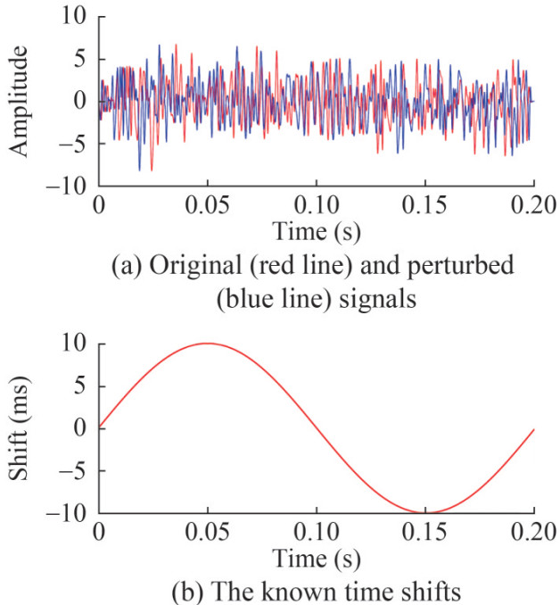Figure  1  Signals and shifts for comparison in noise-free case

Download: Full-Size Img

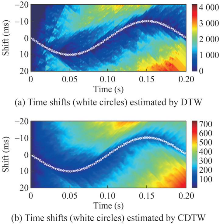Figure  2  Estimated shifts in noise-free case. The white lines represent the known shifts

Download: Full-Size Img

DTW and CDTW provide accurate time shifts in the aforementioned example. However, the field signals display amplitude modulation and noise contamination, which will aggravate the challenges in shift estimation. The original signal (red line) and the amplitude-modulated version (blue line) are shown in Figure 3(a). Multiplying a time-varying factor (Figure 3(b)) to the perturbed signal (Figure 1(a), the blue line) facilitates the generation of the modulated signal. In this case, a clear optimal path is absent on the plot of the distance matrix by conventional DTW (Figure 4(a)). The estimated time shifts by conventional DTW degrade at times around 0.05 and 0.18 s. On the contrary, the amplitude modulation does not affect the CDTW method (Figure 4(b)). The computed distance matrix and estimated time shifts by CDTW are comparable to those in the noise-free case (Figure 2(b)).

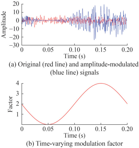Figure  3  Signals and shifts for comparison in amplitude-modulation case

Download: Full-Size Img

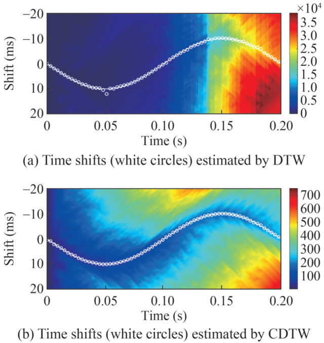Figure  4  Estimated shifts in amplitude-modulation case. The white lines represent the known shifts

Download: Full-Size Img

The performance of conventional DTW and CDTW technologies in the noise contamination case is further compared. The randn() function generates random noise in MATLAB. The random noise is then added to the perturbed signal (Figure 1(a), the blue line). The signal/noise ratio of the noise-contaminated signal (Figure 5(a), the blue line) is 2 dB. The conventional DTW technology severely hinders the noise. No visible optimal path is observed on the distance matrix by conventional DTW. The estimated time shifts by DTW are far away from the actual one in the time range from 0 s to 0.13 s (Figure 5(b), the white circles). Notably, the time shifts reach the artificially set boundary (−20 ms), indicating that conventional DTW unsuccessfully performs in the noise contamination case. By contrast, the noise influence on the CDTW technology is minimal. The estimated time shifts by CDTW fit well with the true one (Figure 5(c), the white circles).

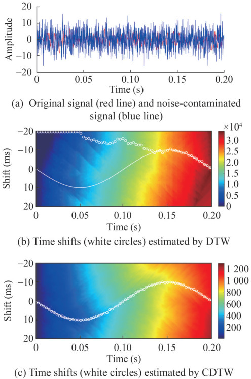Figure  5  Estimated shifts in noisy case. The white lines represent the known shifts

Download: Full-Size Img

The performance of conventional DTW and CDTW technologies in the noise-free, amplitude-modulated, and noise-contaminated cases is compared in this section using high-frequency seismic signals. The presence of amplitude modulation and noise severely affects and contributes to the unstable conventional DTW, thus hindering its use in practical OCCUS applications. By contrast, the CDTW technology can resist amplitude modulation and noise presence. This technology demonstrates promising potential in practical OCCUS applications. The proposed CDTW-FWI will be tested in the next section using numerical experiments.

3   Numerical experiment on the Frio-2 CO₂ storage model

The sources are typically placed near the ocean surface during seismic surveys for monitoring in OCCUS. Meanwhile the receivers are either placed near the ocean surface or down to the ocean bottom. In both cases, the seismic waves propagate through and are affected by the seawater volume. Data processing and quantitative monitoring become increasingly difficult due to this phenomenon. For instance, the images and inversion results are severely degraded by the free-surface multiples (Berkhout and Verschuur, 1997). An alternative to the aforementioned surface sources and receivers is down-well sources and receivers, which can mitigate the seawater influence and are closer to the monitoring target (Daley et al., 2011). Based on previous work (Hovorka et al., 2006; Daley et al., 2007), borehole seismic techniques can image the in situ change in seismic velocity due to the displacement of brine by supercritical CO₂. The effectiveness of the proposed CDTW-FWI method is tested in this section using a cross-well acquisition configuration, in which sources are deployed in a well and receivers in another well far away at an appropriate distance, respectively.

The pressure-wave velocity model is modified upon the Frio-2 CO₂ pilot experiment (Daley et al., 2007). In this small-scale injection experiment, approximately 300 t of supercritical CO₂ are injected into the 17 m-thick Blue sand reservoir at a depth of 1 650 m at the Frio site. The original horizontal and vertical grid intervals are 0.15 m. The original model is discretized on 467×434 grids. The original horizontal and vertical grid intervals are enlarged by an order of magnitude without varying the number of grids (i.e., the grid interval of the modified model is 1.5 m) (Figure (6)).

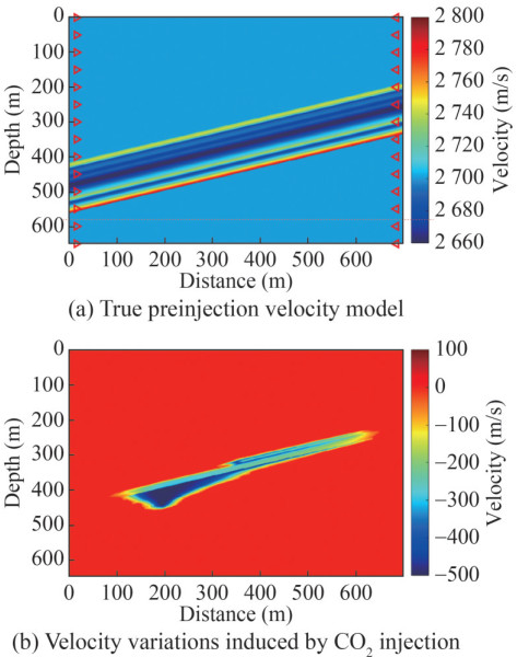Figure  6  Velocity models. The true postinjection velocity is the superposition of panels a and b

Download: Full-Size Img

In the cross-well survey, the source and receiver wells are assumed to be located at x = 15 m and x = 685.5 m, respectively (Figure 6(a)). A total of 109 sources and 217 receivers are evenly deployed in the source and receiver wells, respectively, to record the seismic data. A Ricker wavelet, which has a dominant frequency of 250 Hz, is used as the source term to generate the seismic "observed" data using the pre- and postinjection velocity model (Figure 6). The velocity inside the reservoir varies from 2 650 m/s to 2 765 m/s and is equal to 2 700 m/s outside the reservoir.

In the first stage, the seismic data acquired preinjection are inverted for the baseline model. A homogeneous velocity model of 2 700 m/s is used in this stage as the initial model. The velocity updates by CDTW-FWI are shown in Figure 7(a). The updates fit reasonably well with the baseline model. Conventional FWI is conducted using the CDTW-FWI model to obtain high-resolution baseline velocity. The frequency band from 35 Hz to 500 Hz is used in FWI by a frequency continuation strategy (Bunks et al., 1995). Figure 7(b) shows that the inverted baseline velocity model has high quality.

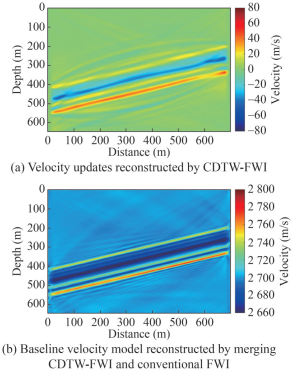Figure  7  Reconstructed velocity models

Download: Full-Size Img

Next, the monitor seismic data for the monitor velocity model are then inverted based on the inverted baseline model.

A crucial component for updating the velocity model is known as the kernel. Figure 8(a) shows the kernel of the first iteration, where the source and the receiver are located at z=199.5 m and z=600 m, respectively. The kernel is superimposed on Figure 6(a). The sensing area of the kernel is clearly depicted in Figure 8(a). This figure highlights the region illuminated by the kernel. Additionally, the travel time of the source–receiver pair will be affected by variations in velocity within the corresponding aquifer area. This finding indicates the feasibility of designing a cost-effective acquisition system with a limited number of sources or receivers. Related work (Daley et al., 2007) has demonstrated that valuable insights into the migration of a CO₂ plume can be obtained using a carefully arranged down-hole source. Figure 8(b) displays the final gradient after summation over 109 sources in the initial iteration. This final gradient effectively emphasizes the low-velocity area induced by CO₂ injection.

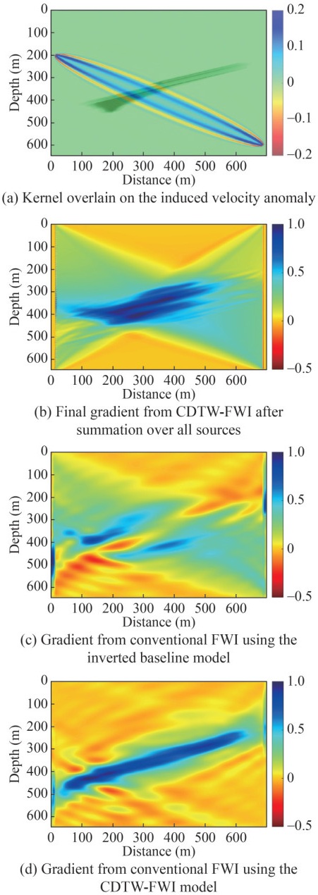Figure  8  Gradients of the first iteration

Download: Full-Size Img

The reconstructed pressure-wave velocity variations by the CDTW-FWI method are shown in Figure 9. The low-velocity area matches well with the truth (Figure 6(b)). The reconstructed result (Figure 9) reveals the high CO₂ saturation area around x=200 m and the narrow low CO₂-saturation area. To some degree, the velocity is underestimated because the travel-time information is sensitive to low- and intermediate-wavenumber velocity variations and not sensitive to the high-wavenumber velocity variations. The evolution of the normalized objective function versus iteration number (Figure 10) illustrates a considerable reduction in the seismic data discrepancy.

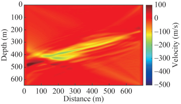Figure  9  Velocity variations reconstructed by the CDTW-FWI method

Download: Full-Size Img

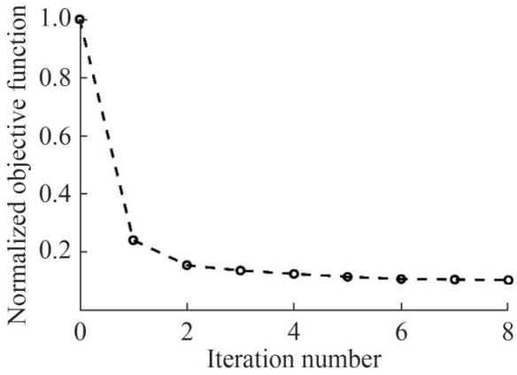Figure  10  Normalized objective function curves versus the iteration number

Download: Full-Size Img

Conventional FWI was performed using different initial models to obtain a high-resolution monitor model. A frequency continuation strategy (Bunks et al., 1995) is adopted from 35 Hz to 500 Hz. Based on the inverted baseline model (Figure 7(b)), the gradient of the first loop from conventional FWI shows an incorrect updating direction (Figure 8(c)). Thus, the inverted velocity model (Figure 11(b)) is far away from the true one (Figure 11(a)), indicating trapping of FWI starting from the inverted baseline model in a local minimum. By contrast, the gradient of the first loop from conventional FWI demonstrates satisfactory updating direction using the CDTW-FWI model inverted from time-lapse data (Figure 9). Starting from the velocity model reconstructed by CDTW-FWI (Figure 9), a high-resolution velocity model is provided by conventional FWI (Figure 11(c)). Figure 11(c) shows the inverted monitor model. If low frequencies (< 35 Hz) are available, then the low wavenumbers of the final result can be further improved. Quantitative estimation of reservoir parameters such as saturation can be established by combining rock physics with the inverted monitor model. The high-resolution velocity variations induced by CO₂ injection can be attributed to the difference between the inverted baseline and monitor models (Figure 11(d)).

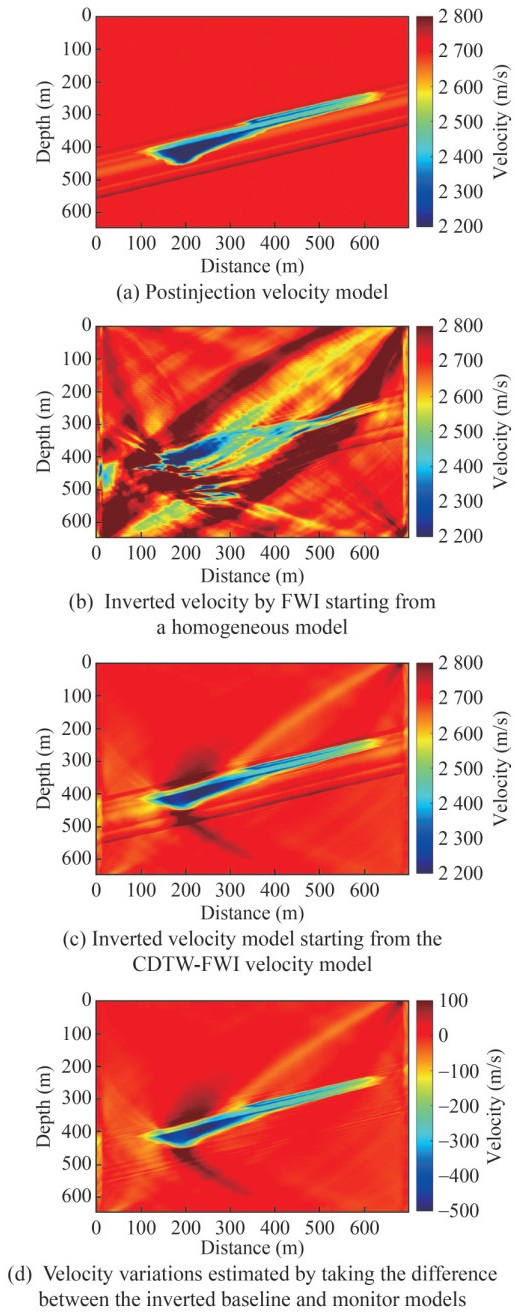Figure  11  Velocity models

Download: Full-Size Img

Finally, Figure 12 reveals the reduction in data differences induced by CO₂ injection using the proposed CDTW-FWI method. A remarkable data difference is observed between the monitor shot gathers and the shot gathers simulated using the homogeneous model (Figure 12(a)). A substantial reduction in the discrepancy between the monitor data and the data simulated using the inverted baseline model is observed after the first stage inversion (Figure 12(b)). As shown in Figure 12(c), the computed waveform using the inverted monitor is close to the true monitor data, indicating the successful estimation of velocity changes.

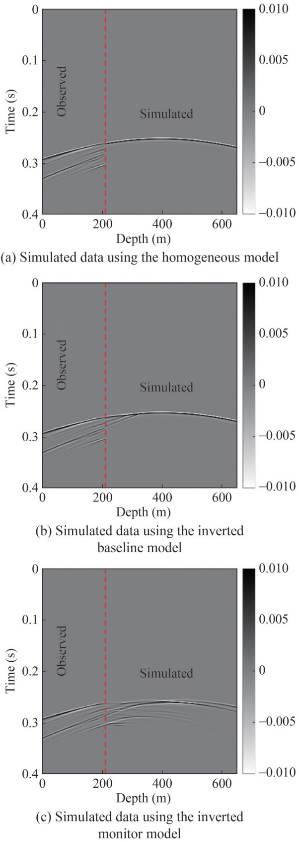Figure  12  Comparison between simulated data and observed data

Download: Full-Size Img

4   Conclusions

The time-lapse CDTW-FWI method was applied to facilitate the inversion of seismic data and estimation of velocity models for CO₂ sequestration monitoring. The cycle-skipping problem was effectively addressed through this method, and the velocity variations due to CO₂ injection were accurately reconstructed. High-resolution velocity models were obtained by combining CDTW-FWI with conventional FWI methods. The obtained results on pairs of signals demonstrate that CDTW can accurately measure the data discrepancy due to CO₂ injection, even in cases of amplitude modulation and noise contamination. Furthermore, the effectiveness of the CDTW-FWI method was proven through numerical experiments on the Frio-2 CO₂ storage model. Thus, future research should focus on the application of the proposed method to field OCCUS seismic data.