
Characterization of Depleted Hydrocarbon Reservoir AA-01 of KOKA Field in the Niger Delta Basin for Sustainable Sub-Sea Carbon Dioxide Storage
https://doi.org/10.1007/s11804-024-00464-9
-
Abstract
This study characterized the AA-01 depleted hydrocarbon reservoir in the KOKA field, Niger Delta, using a multidimensional approach. This investigation involved data validation analysis, evaluation of site suitability for CO2 storage, and compositional simulation of hydrocarbon components. The primary objective was to determine the initial components and behavior of the hydrocarbon system required to optimize the injection of CO2 and accompanying impurities, establishing a robust basis for subsequent sequestration efforts in the six wells in the depleted KOKA AA-01 reservoir. The process, simulated using industry software such as ECLIPSE, PVTi, SCAL, and Petrel, included a compositional fluid analysis to confirm the pressure volume temperature (PVT) hydrocarbon phases and components. This involved performing a material balance on the quality of the measured data and matching the initial reservoir pressure with the supplied data source. The compositional PVT analysis adopted the Peng–Robinson equation of state to model fluid flow in porous media and estimate the necessary number of phases and components to describe the system accurately. Results from this investigation indicate that the KOKA AA-01 reservoir is suitable for CO2 sequestration. This conclusion is based on the reservoir's good quality, evidenced by an average porosity of 0.21 and permeability of 1 111.0 mD, a measured lithological depth of 9 300 ft, and characteristic reservoir – seal properties correlated from well logs. The study confirmed that volumetric behavior predictions are directly linked to compositional behavior predictions, which are essential during reservoir initialization and data quality checks. Additionally, it highlighted that a safe design for CO2 storage relies on accurately representing multiphase behaviour across wide-ranging pressure–temperature–composition conditions.-
Keywords:
- Carbon capture ·
- CO2 sequestration ·
- Geological storage ·
- Geo-mechanical modeling ·
- Multiphase flow ·
- Niger Delta
Article Highlights• Offshore geologic settings worldwide provide high volume of storage capacity needed to reduce CO2 emissions at global scale.• Characterizing potential CO2 storage sites is critical to ensuring the integrity and safety of a CO2 storage scheme, making site selection for a CCS chain critical.• This study involved data validation analysis, evaluation of site suitability for CO2 storage, and compositional simulation of hydrocarbon components using industry software such as ECLIPSE and PETREL.• The result from the simulation indicates that the KOKA AA-01 reservoir is suitable for CO2 sequestration. -
1 Introduction
Carbon dioxide (CO2) sequestration, also known as carbon dioxide capture and storage (CCS), is among the most effective technologies to mitigate the effect of greenhouse gas emissions and combat climate change. The continuous rise in Earth's temperature owing to hydrocarbon utilization can be significantly reduced through this method (Lackner, 2003; Pacala and Socolow, 2004). If fully implemented, CCS could potentially reduce global hydrocarbon emissions by 20% by 2050 and by 55% by the end of the century (Metz et al., 2005). The CCS process involves capturing CO2 from primary stationary sources, transporting it via pipelines, and injecting it into appropriate deep geological formations to prevent its release into the atmosphere (Bachu et al., 2007). Specifically, CO2 sequestration involves capturing and transporting CO2 from anthropogenic sources and then injecting supercritical CO2 into underground geologic formations (Figure 1). This method not only reduces carbon emissions but also facilitates CO2 storage and utilization on the seabed, employing pipelines or ships to transport captured CO2 to permanent storage sites such as depleted hydrocarbon reservoirs and saline aquifers or by injecting it to replace and displace subsea resources (Figure 2). Earth's carbon reservoirs include carbonate reservoir rocks, coals, oil and gas reservoirs, and organic-rich shales.
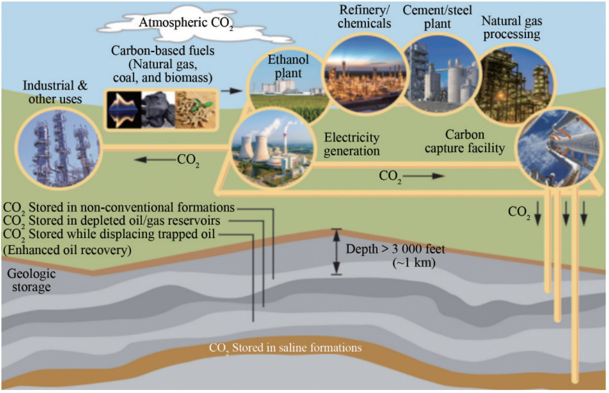 Figure 1 Carbon capture, use, and storage supply chain (Source: Rocky Mountain Coal Mining Institute. Atlas iv, 2012)
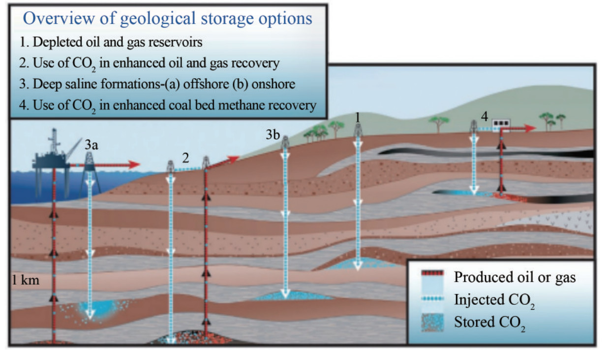 Figure 2 Carbon dioxide storage options (Orr, 2009)
In Nigeria, CO2 emissions are primarily anthropogenic, driven largely by industrial activities and gas flaring in the Niger Delta region owing to oil and gas exploration and exploitation. The industrial revolution of the 19th century, which saw extensive fossil fuel use, contributed significantly to these emissions. Natural resources are used extensively in construction, industries, transportation, and household consumption (Badru, 2020). Human activities have accelerated climate change, with scientific consensus indicating that human activity is very likely the cause of the rapid increase in global average temperature over the past several decades. The consequences of climate change in Nigeria are severe, including irregular rainfall patterns, which may sometimes be excessive. Irregular rainfall can lead to excessive rainfalls, causing flooding that devastates people and properties. For example, in 2002, more than 16 states experienced catastrophic flooding, resulting in numerous deaths and the displacement of over 2 million people (Badru, 2020).
In this study, CCS comprises capturing CO2 from stationary sources, compressing it into a supercritical fluid, and re-injecting it into deep geological formations for long-term storage (Orr, 2009). CCS is essential since it allows the continuous use of hydrocarbons, which presently supplies over 80% of the primary energy while offering significant emission mitigation compared to other technologies (Hoffert et al., 2002).
Key to successful CCS implementation is identifying geologic formations with sufficient pore space (porosity) in which CO2 can be contained for storage and pathways connecting these pores (permeability) to enable effective CO2 injectionand movement (Eigbe et al., 2022). Characterizing potential CO2 storage sites is critical to ensuring the integrity and safety of a CO2 storage scheme, making site selection for a CCS chain critical.
Abandoned hydrocarbon fields, considered uneconomic for further production, are suitable sites for CO2 underground storage. The geological characteristics crucial for storage sites are comparable to those used for underground storage. The depleted hydrocarbon fields have been extensively characterized during the exploration and production phases, making them suitable for geological storage owing to their proven capability to trap hydrocarbon over long periods (Ajayi et al., 2019). Numerical models of comparable underground formations that were previously history-matched provided insights into the geological environment. Wells and infrastructures used for hydrocarbon production from depleted fields could be repurposed for CO2 injection. Determining optimum injection pressures is important to avoid exceeding the caprock's pressure limits, which could result in CO2 leakage from the abandoned wells, especially around the back of well casings. This significantly limits the practical storage capacities of depleted reservoirs.
Extensive research has been conducted on the viability of CO2 underground storage in depleted hydrocarbon reservoirs worldwide (Zhou et al., 2020; Mkemai and Gong, 2020; Raza et al., 2017). The studies have shown that depleted hydrocarbon reservoirs are well characterized and outlined over long periods of research and production. The reservoirs have demonstrated the capability to hold buoyant fluids, with model outputs indicating that CO2 injection can facilitate the production of additional CH4 (Oldenburg et al., 2001). A review by Eigbe et al. (2023) indicated that injectivity and trapping mechanisms are significantly affected by precipitation (Raza et al., 2017; Shariatipour et al., 2016). However, the review found that authors could not correctly explain CO2 plume behavior below sealing rocks and, therefore, suggested a more focused approach to investigate this phenomenon to validate these predictions.
This study involves reservoir characterization by applying a multidimensional method, including compositional simulations and analyses of different hydrocarbon components in the Niger Delta basin subsea. This area has not been sufficiently studied, possibly owing to the complexities involved. The relevance of this approach to reservoir characterization lies in the fact that it considers possible interactions among other hydrocarbon fluid components when CO2 is injected into geological formations for storage. In essence, these interactions could lead to undesired leakages during CO2 sequestration. The focus of this study is on reservoir characterization through compositional simulations of various hydrocarbon components using six wells (Koka-01, Koka-02, Koka-03, Koka-04, Koka-05ST1, and Koka-05ST2) in the KOKA AA-01 field in the Niger Delta as a test case.
2 Background of the geology and CO2 storage in the niger delta
2.1 Geological setting of the niger delta
The Niger Delta basin is situated around the Gulf of Guinea and covers the entire Niger Delta area (Klett et al., 1997). The delta prograded southwest from the Eocene to the present, creating depobelts that characterize the most active areas of the delta during its development stages (Doust and Omatsola, 1990). These depobelts developed into one of the world's major regressive deltas, covering approximately 300 000 km2 (Kulke, 1995), with a sediment volume of 500 000 km3 (Hospers, 1965) and a sediment thickness exceeding 10 km in the basin depocenter (Kaplan et al., 1994).
According to Kulke (1995), there is only one recognized petroleum system in the Niger Delta: the Tertiary Niger Delta (Akata-Agbada) Petroleum System. This system's highest range corresponds with the province boundaries, while its minimum extent is defined by the area coverage of the oil fields. It comprises identified resources (aggregate production and proved reserves) totaling 34.5 billion barrels of oil (BBO) and 93.8 trillion cubic feet of gas, equivalent to 14.9 billion barrels of oil equivalent. Presently, most of the oil is found in onshore fields or on the continental shelf in waters less than 200 meters deep, predominantly in large, relatively simple structures. A few giant fields exist within the delta, the largest of which comprises just over 1.0 BBO (Petro Consultant, 1996).
The Niger Delta onshore area is described by the geology of Southern Nigeria and south western Cameroon. The northern border is marked by the Benin flank, an east-north-east trending hinge line south of the West Africa basement massif. The north-eastern border is defined by Cretaceous outcrops on the Abakaliki High, extending southeast to the Calabar flank, a hinge line adjoining the nearby Precambrian terrain.
The offshore section of the Niger Delta area is bounded by the Cameroon volcanic line to the east, the eastern border of the Dahomey Basin (the easternmost West African transform-fault passive margin) to the west, and the 2 km sediment thickness contour or the 4 000 m bathymetric contour in sections where sediment thickness exceeds 2 km to the south and southwest. This region spans about 300 000 km2 and comprises the geologic extent of the Tertiary Niger Delta (Akata-Agbada) Petroleum System, as illustrated in Figure 3.
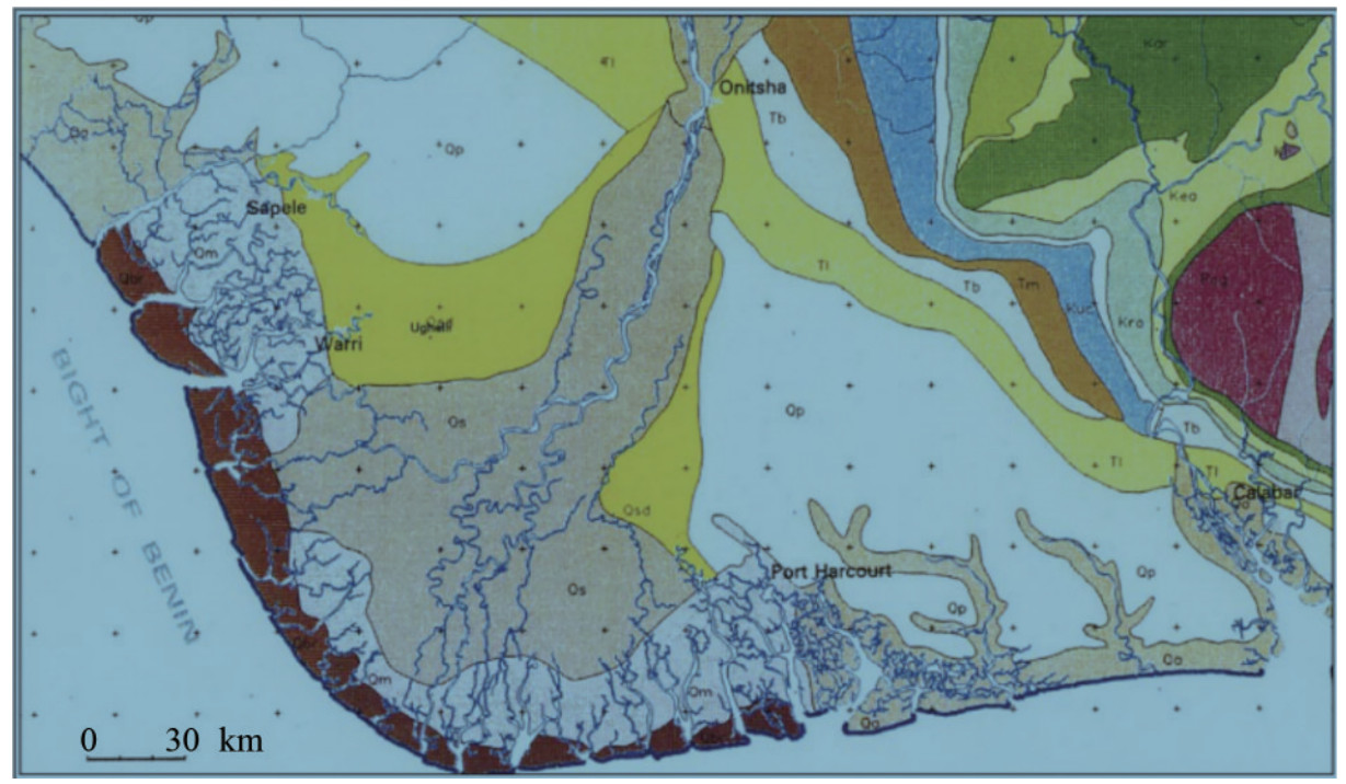 Figure 3 Geological map showing the Niger Delta and environs (Whiteman, 1982)
2.2 Lithostratigraphy of niger delta
The Tertiary unit of the Niger Delta is divided into three formations, characterized by prograding depositional facies distinguished primarily based on sand-shale ratios, as shown in Figure 4. These formations are documented in different papers (Avbovbo, 1978; Doust and Omatsola, 1990; Kulke, 1995).
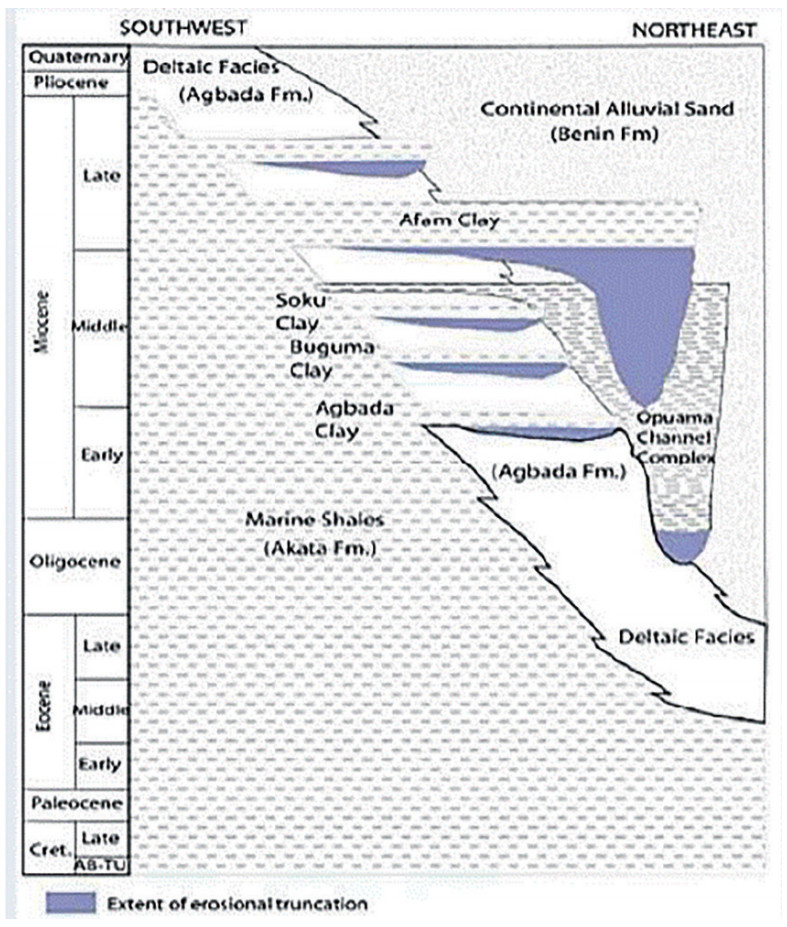 Figure 4 Stratigraphic column of the Niger Delta basin. Modified from Doust and Omatsola (1990)
The Akata formation at the lower part of the delta is of marine origin. It comprises thick shale sequences (potential source rock), turbidite sands (potential reservoirs in deep water), and minor amounts of clay and silt. Formed from the Paleocene to the Recent, the Akata formation developed during low stands when terrestrial organic matter and clays were transported to deep water areas characterized by low energy conditions and oxygen deficiency (Stacher, 1995). The top of the Akata Formation is considered the economic basement for oil exploration and production.
The Agbada formation consists of a paralic succession of alternating sandstones and shales. The sandstones within this formation are the primary reservoirs for oil and gas in the Niger Delta (Doust and Omatsola, 1990). The formation consists of an alternating sequence of sandstones and shales of delta-front, distributary-channel, and deltaic-plain origins. The sandstones are medium to fine-grained, clean, locally calcareous, glauconitic, and shelly. The shales are medium to dark gray, fairly consolidated, and silty with local glauconite. In this formation, the sand beds serve as the main hydrocarbon reservoirs, while the shale beds form the cap rock.
The Benin Formation is composed of continental sands from Eocene to Recent deposits. These alluvial and upper coastal plain sands can be up to 2 000 m thick (Avbovbo, 1978). The composition, structure, and grain size of the sequence indicate deposition of the formation in a continental, probably upper deltaic environment. The age of the formation varies from Oligocene (or earlier) to Recent (Avbovbo, 1978). The Benin Formation also serves as the aquifer in the Niger Delta.
2.3 Necessity for CO2 sequestration in the niger delta
Burning fossil fuels has led to the emission of CO2 as the main greenhouse gas into the atmosphere. Gas flaring and venting produce CO2, methane, and other gases that increase the concentration of greenhouse gas (GHG) emissions, resulting in the depletion of the ozone layer and negatively affecting the global environment. This contributes significantly to global warming and climate change (U. S Environmental Protection Agency, 2015). Nigeria is among the top countries responsible for 75% of global gas flaring emissions, flaring 16% of the total associated gas with a conservative estimate of 56.6 million m3 (World Bank, 2004; Ishisone, 2004). Global climate change, driven by escalating GHG emissions, is one of the most pressing challenges of our time. In Nigeria, the rise in GHG concentrations, particularly CO2, fundamentally alters the Earth's climate, leading to various adverse effects, including rising temperatures, extreme weather events, and sea-level rise (Masson-Delmotte et al., 2021). Man-made emissions of GHGs have increased by 70% from 29 Gtons of CO2 equivalent (GtCO2e) in 1970 to 49 GtCO2e in 2004, with 25.8 Gtons of CO2 emissions coming from fossil fuel combustion (OECD/ITF, 2009). In developing countries like Nigeria, particularly in Lagos (Nigeria), automotive emissions, power plants, factories, and other stationary sources contribute to the increase in GHG emissions owing to high levels of traffic and industrialization (OECD/ITF, 2009). The Niger Delta, covering an estimated area of 75 000 km3, has the largest flaring activities, significantly contributing to environmental problems such as increased atmospheric temperature (Oseji, 2007; Sonibare et al., 2008). Over a period of 49 years, gas flaring activities in the Niger Delta have emitted an estimated 4.56×10⁸ tons of CO2 equivalent into the atmosphere, corresponding to a yearly emission of 9 315.46 tons in the region (Giwa et al., 2014). A consideration of countries with high emission levels and sequestration capacity shows that some of the greatest CO2 emitters are located in regions with substantial sequestration potential. This requires CCS initiatives, which will likely begin in regions with large emission sources and sequestration potential.
2.4 Geological conditions for CO2 storage
When selectinga suitable geological site for CO2 storage, three major conditions must be met: storage capacity, injectivity, and containment. The selected geological site's storage capacity must havea suitable pore pace to accommodate large volumes of injected CO2. This requires the site to exhibit excellent porosity and/or cover a substantial area. Optimal injectability is achieved when the geological formation allows for lower wellhead pressures to maintain desired injection rates. A high permeability value makes the selected geologic formation a good candidate for CO2 injectivity. Another essential requirement is the presence of suitable cap rocks and sealing faults that guarantee that they prevent the injected CO2 from escaping to the atmosphere or leaking into underground water sources. CO2, having a lower density than the original brine in place, must be contained effectively to avoid leakage.
For successful storage, CO2 should be stored in a supercritical state, achieved by compressing it to higher pressures and temperatures (about 89 °F and 7.4 MPa). In such a state, CO2 exhibits the characteristics of a liquid but flows like a gas, significantly decreasing the buoyancy disparity between the CO2 and in situ fluids (Grobe et al., 2009).
3 Materials and methods
3.1 Primary and secondary variables for the system under study
Primary variables determine the system's thermodynamic equilibrium and are typically solved directly during the simulation. In this context, the primary variables for this study are the following:
1) Pressure (P): The pressure of each phase (oil, gas, and brine) in the reservoir.
2) Temperature (T): The temperature within the reservoir. Secondary variables are derived from the primary variables and provide additional information about the system. They are not directly solved in the governing equations but are computed from the primary variables. Standard secondary variables in reservoir simulations and CO2 sequestration include phase compositions, pressure gradients, and temperature gradients.
Phase compositions: The compositions of each component (oil, water, CO2, and CH4) in each phase (oil, gas, and brine) are calculated based on phase equilibrium models or state equations.
Saturation: The fraction of each phase (oil, gas, and brine) in a specific reservoir volume, calculated based on the fluid properties and phase behavior.
Pressure and temperature gradients: Pressure and temperature slopes in the reservoir are applied to understand fluid flow, heat transfer, and pressure variations.
Phase properties: Various thermodynamic properties of each phase (density, viscosity, and compressibility) are derived from the primary variables using equations of state or correlations.
Phase mobility and relative permeability: The mobility and relative permeability of each phase depend on the phase saturations and are essential for describing flow behavior.
3.2 Determination of independent state variables
The thermodynamic system in this study can be described unambiguously by a set of state variables that are independent of each other. To determine the number of independent state variables required to describe the system involves applying Gibb's rule to a non-isothermal three-phase four-component system (oil, gas, brine, and components: oil, water, CO2, and CH4). Gibbs' phase rule states:
$$ F=C-P+2 $$ (1) where F is the degrees of freedom (number of independent state variables), C is the number of components in the system, and P is the number of phases in the system.
In the given system, we have: C = 4 components (oil, water, CO2, and CH4), P = 3 phases (oil, gas, and brine). Calculating the degrees of freedom, F = 3.
This indicates hat in a non-isothermal three-phase, four-component system comprising oil, gas, and brine, and the component composition, namely oil, water, CO2, and CH4, three independent state variables must be solved to fully describe the system. These state variables could be the pressure, temperature, and composition (mole fractions) of the components in each phase.
3.3 Mathematical relations for primary and secondary variables
The mathematical relations utilized to express the phase state of the reservoir fluid components and the associated primary and secondary variables applied for this study are outlined in Table 1. In this table, the phase state "oil phase" refers to the presence of only a single oil-rich phase. Similarly, "gas phase" indicates the presence of only a gas-rich phase, while "brine phase" refers to the presence of only a brine-rich phase.
Table 1 Primary and secondary variables with phase changesS/N Phase state Present component Primary variables Secondary variables (Phase vhanges) Oil phase appearance Gas phase appearance Brine phase appearance 1 All 3 Phases (Oil, Gas and Brine) O, W, CO2, CH4 P, T, Sw, p_i, µ_i, B_i, cp_i, k_i K_i, ϕ_i, ∇P, ∇T nil nil nil 2 2 Phases (Brine and Gas) W, CO2, CH4 P, T, Sw, p_i, µ_i, B_i, cp_i, k_i nil x_gas>0
$X_b^g \geqslant\left(X_b^g\right) \max$X_brine>0
$X_g^b \geqslant\left(X_g^b\right) \max$3 2 Phases (Oil and Brine) O, W P, T, Sw, p_i, µ_i, B_i, cp_i, k_i x_oil>0
$X_b^o \geqslant\left(X_b^o\right) \max$nil X_brine>0
$X_o^b \geqslant\left(X_o^b\right) \max$4 2 Phases (Oil and Gas) O P, T, Sw, p_i, µ_i, B_i, cp_i, k_i x_oil>0
$X_g^o \geqslant\left(X_g^o\right) \max$x_gas>0
$X_o^g \geqslant\left(X_o^g\right) \max$nil 5 Brine Phase W P, T, Sw, p_i, µ_i, B_i, cp_i, k_i nil nil $\mathrm{x}_{\mathrm{gas}}<0>\mathrm{x}_{\text {_oil }} \\ \text { X_brine }>0$ 6 Oil Rich Phase O P, T, S, p_i, µ_i, B_i, cp_i, k_i xgas<0>x_brine
x_oil>0nil nil 7 Gas Rich Phase CO2, CH4 P, T, S, p_i, µ_i, B_i, cp_i, k_i nil xoil<0>x_brine
x_gas>0nil Equations of state are critical for forecasting or equating the fluid phase behavior in complex systems, such as hydrocarbon fluid components in oil and gas reservoirs. Successful simulations depend on extrapolating the number and the compositions of phases existing at a given pressure, temperature, and overall fluid composition using Gibbs energy analysis of phase equilibria.
Regarding fluid saturations or relative permeability, the hydrocarbon reservoir can be divided into two regions. Single-phase regions represent areas in the P – T diagram where each component or phase can exist alone, while two-phase regions represent areas where two phases coexist, typically termed vapor and liquid. It is crucial to note that the liquid state may include water and oil, which makes it a phase system with fluid mobility determined by the critical point. In this study, oil and gas initially exist under undersaturated oil conditions and then separate at the saturation pressure. The phase diagram generated after matching the initial conditions of the fluid in PVTi is shown in Figure 5. The critical temperature and pressure were estimated as 802.91 °F and 1 570.12 psia, respectively. In addition to the injection depth, these vital conditions are crucial in designing the CO2 injection and sequestration system (Sengul, 2006). To maintain accuracy in the simulation, a material balance validation is performed on the data subsequently.
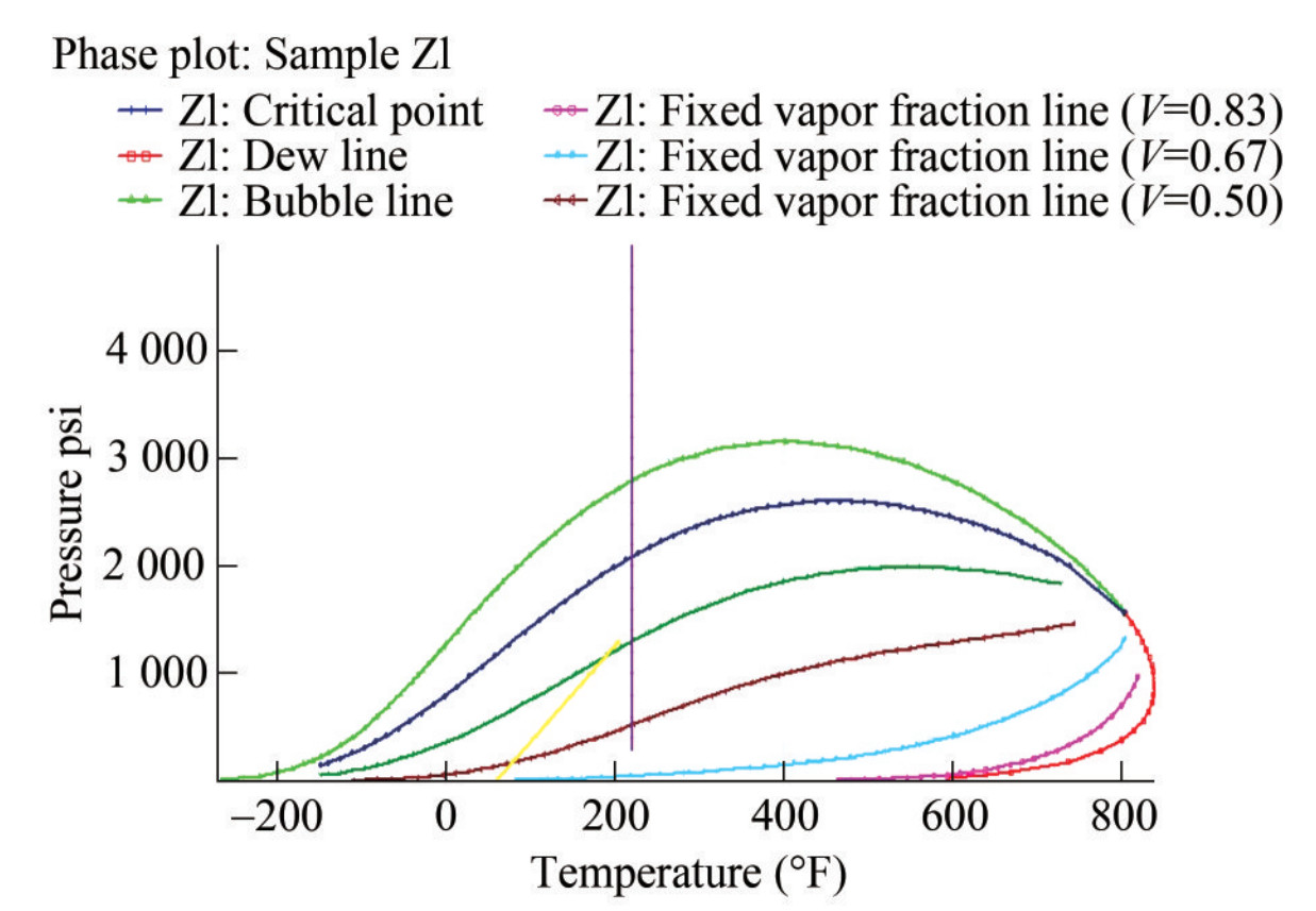 Figure 5 Phase diagram matching the initial conditions of fluid in PVTi
3.4 Data set and analysis
This study's major data set is derived from the static model for the KOKA AA-01 reservoir. The primary parameters included in this model are grid dimensions, facies, zones, horizons, wells, and well tops. The data does not include fluid and rock properties like oil-water contact (OWC), gas-oil contact (GOC), datum depth, oil PVT, and gas PVT. However, it included well logs from five (05) wells, well data like their coordinates and deviations, and well logs including neuron logs, resistivity, gamma ray, and spontaneous potential. Other data utilized in this study included contacts, SCAL data, initial pressure/pressure data, and separate PVT data. A detailed data set for this study is shown in Table 2.
Table 2 List of data and validation proceduresS/N File Remark Format Parent folder Provided as Validation 1 Static Model The entire geologic model can help confirm the given input data in PETREL. PG 1. KOKA Petrel Project.ptd
2. KOKA Petrel Project.petWas loaded into Petrel and model confirmed. 2 GRID The ASCII format is preferable ASCII (*GRDE CL) and BINARY (*GRID, *EGRID) formats. Same as 1 above Same as 1 above Same as 1 above 3 PVT Data Reservoir Formation Test if available will suffice PDF or EXCEL RE KOKA.PVT.xlsx 1. Conclusively validated by Model Initialization
2 Indicates crude is undersaturated Oil
3 Indicates Initial Pressure, Pi@4056 psia4 Well Data Well Logs, etc ASCII or EXCEL PP Koka-001.asc, Koka-002.asc, Koka-003.asc, Koka-004.asc, Koka-005.asc, Loaded in a separated model and still confirmed in the given static model 5 Contacts OWC/GOC logged from respective wells ASCII or EXCEL PP Koka Reservoir Average.xlsx To be loaded in PETREL, and ECLIPSE as a final confirmation 6 SCAL Data Relative Permeability and Capillary Pressure Any of ASCII, EXCEL, and PDF RE 1 Koka_SCAL_Kr_PC.xlsx Loaded in PETREL, and ECLIPSE as and confirm to have different classes of Rel Perm endpoint for Oil/Water. 7 Initial Pressure/Pressure Data RE KOKA.PVT.xlsx, Koka_Production_Pressure.xlsx Validated during initialization in Petrel and Eclipse 8 Production History Data Example, 30 years of Oil and Gas production up to depleted (mature stage). With/Without CO2 Recovery. ASCII or EXCEL PT Koka_Production_Pressure.xls/Koka Well Production To be loaded in PETREL and ECLIPSE as a final confirmation. The data from the reservoir static model and the suite of separate data, as highlighted above, were analyzed using specialized modeling software, Petrel 2022. This software provides a transparent correlation canvas that integrates various types of data over time. Key features include seismic data integration, grid data visualization, log data correlation, core image display, even completions, and simulation outputs.
3.5 Reservoir fluid compositional analysis
3.5.1 Compositional fluid simulation
The compositional simulation was conducted to understand the variation in petrophysical properties with depth, the hydrocarbon fluid variation with depth, and the distribution of the petrophysical reservoir model. This simulation utilized parameters outlined in Tables 3 and 4 and was performed using ECLIPSE 300. The hydrocarbon fluids in this study comprise both hydrocarbon and non-hydrocarbon constituents, ranging from light molecular weight components like CH4 to heavier fractions (Igwe et al., 2020). The compositions of these constituents in oil and gas states vary owing to specific reservoir conditions like temperature and gravity. Understanding fluid behavior at surface and reservoir conditions, along with the compositions and constituents of reservoir fluids, is critical. This entails recognizing the causes and practices influencing fluid behavior. The above responsibilities could be accomplished through reservoir simulation practice, and these will also assist in the efficient production of petroleum reservoir fluids from the reservoir to the ground level.
Table 3 Reservoir parametersParameter Value Initial reservoir pressure (psia) 4 056 Reservoir temperature (°F) 177 Range of porosity values 0.11–0.27 Mean porosity 0.21 Average permeability value (mD) 1 111.0 Maximum number of wells 0 Maximum number of separators 5 Grid dimension (ft3) 50×42×63 Total grids cells 132 300 Reservoir crest (ftss) 9 238 OWC (fts) 9 314 Hydrocarbon column (ftss) 76 Table 4 Initialized volume of reservoir fluidsFluid Component Value Oil (Res Vol) (fb) 0 Water (Res Vol) (rb) 9 374 013.1 Gas (Res Vol) (rb) 51 854 046 Water (Surf Vol) (stb) 9 477 775.2 Oil (wrt separator) (stb) 1.897 465 2×10⁸ Gas (wrt separator) (Mscf) 0 There is an assumption that compositions of the several fluid constituents are similar in all areas around the reservoir system in many compositional reservoir simulation operations like this study. Conversely, the assumption of constant composition is improper and impracticable because it completely ignores the phenomenon of certain less obvious physical procedures in some reservoirs, as revealed in recent studies. Factors like thermal diffusion, temperature variation with depth, gravitational force, and others contribute significantly to the spreading and variation in hydrocarbon fluid compositions within the reservoir (Bogatyrev et al., 2015). The compositional variation in the KOKA AA-01 reservoir increases variations in fluid characteristics like molecular weight, density, gas-oil ratio (GOR), and saturation pressure (Pedersen and Hjermstad, 2015).
For this study, it is necessary to initialize the existing reservoir simulation model with a compositional gradient model that sufficiently describes the elements causing the compositional gradation in the reservoir system and properly calculates in-place volumes and reservoir performance. Existing literature shows little application of compositional gradient models for reservoir model initialization, with the isothermal compositional gradient model being the primary compositional gradient model used to achieve this goal (Jaramillo and Barrufet, 2001; Vo and Horne, 2015).
Research has shown that relying solely on gravity influence and constant temperature theories in isothermal compositional gradient models is inadequate. Temperature variations and thermal diffusion also significantly contribute to compositional gradations relative to depth in the reservoir (Pedersen and Hjermstad, 2015; Nikpoor et al., 2013). Furthermore, few publications exist on reservoir models initialized with compositional gradient models (specifically, non-isothermal compositional gradient models) that accurately account for all factors causing compositional gradients in hydrocarbon reservoirs. This gap in knowledge highlights the need for advanced modeling approaches. Consequently, this study utilizes the compositional gradient models, which sufficiently account for the discrete and mutual resultant effects of thermal diffusion, gravitational forces, and temperature gradients, to initialize reservoir simulation models.
3.5.2 Equation of state for hydrocarbon mixtures
A classic hydrocarbon consists of millions of individual components. The equation of state used to model the phase behavior of this mixture utilizes values for parameters A and B.
For instance, the Peng-Robinson equation of state is stated as follows:
$$ P=\frac{R T}{V-B}+\frac{A}{V(V+B)+B(V-B)} $$ (2) This reservoir simulation approach uses about four components and pseudo-components to describe the mixture. Each component has associated values for Tc, Pc, Vc or Zc, ω, Ωa, and Ωb. Additionally, binary interaction coefficients δij, which modify the forces among component pairs, must be determined during fluid description analysis. The quantified parameters are normally considered fixed for pure components like nitrogen or CH4. However, to ensure that the estimated phase aligns with experimental data, the residual component factors need to be changed. This phase behavior equilibration practice is conducted using the PVT i software (Chang et al., 1998).
The next step involves applying ECLIPSE 300 to define the volume of liquid and phase compositions in a single grid at equilibrium. ECLIPSE 300 employs linear, non-linear (Newton), and flash programs to achieve a converged solution. After each time step, the output for every grid block comprises oil and gas saturations, water, pressure, and oil mole fractions of each component in the liquid and vapor phases, and liquid and vapor molar fractions.
A stability test was carried out to determine the number of hydrocarbon phases present. If three hydrocarbon phases are identified, as is applicable in this study, K-values, Ki, are assigned to each component, i.
These values are either derived from the former iteration or obtained using Wilson's formula:
$$ K_i=\frac{\mathrm{e}^{\left[5.37\left(1+\omega_i\right)\left(1-\frac{1}{T_{n i}}\right)\right]}}{P_{r i}} $$ (3) Then, given zi and Ki, ECLIPSE 300 solves the flash equation to produce the molar portion of vapor, V. The flash equation solved by ECLIPSE 300 is as follows:
$$ g(V)=\sum\limits_{i=1}^{N_{\text {coms }}} \frac{z_i\left(K_i-1\right)}{1+V\left(K_i-1\right)}=0 $$ (4) ECLIPSE 300 solves this equation to obtain the mole portions of every component in the liquid and vapor phases:
$$ x_i=z_i /\left[1+V\left(K_i-1\right)\right], i=1, 2, \cdots, N_{\text {comps }} $$ (5) $$ y_i=\left(K_i z_i\right) /\left[1+V\left(K_i-1\right)\right], i=1, 2, \cdots, N_{\text {comps }} $$ (6) Applying these mole fractions, the Peng-Robinson equation of state could be stated as a cubic equation of the compressibility factor Z:
$$ Z^3-Z^2(1-b)+Z\left(a-3 b^2-2 b\right)-\left(a b-b^2-b^3\right)=0 $$ (7) where Z is defined by $Z=\frac{P V}{R T}$, and the two remaining parameters are defined by:
$$ a=\frac{A P}{R^2 T^2} $$ (8) $$ b=\frac{B P}{R T} $$ (9) The solution of this above cubic equation is given in a two-phase region with three real roots. The largest root represents the compressibility factor of the vapor phase, and the smallest positive root indicates the compressibility factor of the liquid phase. The ECLIPSE 300 iteration uses these compressibility factors to calculate the fugacity of every component in the liquid and vapor phases (Chang et al., 1998).
3.6 Model initialization
The initialization of the reservoir using equilibration was conducted with the ECLIPSE 300 tool. The primary goal of this initialization was to determine the initial conditions in the model and ensure that the reservoir reached hydrostatic equilibrium before starting the simulation. The reservoir model was successfully initialized, with all fluid properties at static equilibrium, indicated by an oil mobility ratio of zero. The simulation also provided the initial values of the oil and gas originally in place. Dynamic models are standard tools in reservoir engineering for generating production profiles and carrying out robust reservoir characterization. Constructing and initializing 3D dynamic reservoir models is challenging owing to the complex prerequisites, which involve using subsurface data across different scales (rock and fluid) and iterative algorithms h. Proper initialization is critical for 3D dynamic reservoir models to accurately distribute the reservoir fluid and estimate the original hydrocarbons in place.
The first run of the initialization process aims to identify data entry errors. This step determines the pressure, fluid saturation distribution, and fluid volumes in place for different fluids inside the reservoir. The results of this initial run will guide the subsequent steps in the 3D dynamic modeling process. A good definition of the reservoir rock types is necessary to develop proper saturation distribution at the model's initial conditions. Processes related to model initialization processes include rock typing, model grid design (Guo et al., 2007), and incorporating additional data such as fluid contacts, fluid properties (PVT), capillary pressure profiles, reservoir thickness, and relative permeability curves. The efficiency of a hydrocarbon reservoir simulator is determined by how dependable the initialization process is, which is controlled by the quality of the reservoir modeling and its realization (Yemez et al., 2013). The Standard assessments of initialization ensure accurate volumetric distributions of fluids around the grid cells that represent the reservoir at its initial condition and anticipated hydrostatic equilibrium (Carlson, 2006).
This study demonstrates an approach based on a dynamic model for characterizing depleted hydrocarbon in the Niger Delta area for CO2 underground storage.
3.7 Reservoir characterization
This study involved the characterization of reservoir properties to assess the feasibility of carbon sequestration, emphasizing storage capacity and injectivity. This involved evaluating the reservoir capacity to receive the projected volume of CO2 and its ability to allow CO2 injection at the rate provided by the CO2 emitters. This assessment was based on data obtained from well logs prior to implementing these practices:
1) Wireline logs, consisting of resistivity logs, neutron logs, gamma-ray logs, and spontaneous potential logs, were applied to determine the rock type and reservoir delineation.
2) In addition to other experimental relationships, data from the analyzed well logs aided in quantitatively describing important reservoir properties.
3.7.1 Calculation of reservoir storage capacity
Estimating the theoretical storage capacity of CO2 for sequestration is crucial for determining the amount of CO2 that can be sequestered in a hydrocarbon reservoir (Ojo and Tse, 2016). In this study, the storage capacity of the KOKA AA-01 reservoir is estimated according to methods outlined by NETL (2007) and Davis et al. (2018):
$$ M_{\mathrm{CO}_2}=A \times h_n \times \phi_e \times\left(1-S_w\right) \times B_o \times \rho_{\mathrm{CO}_2} \times E $$ (10) where MCO2 is the mass estimate of the underground reservoir CO2 storage capacity, megaton (MT); A is the area of reservoir accessed for CO2 storage capacity estimation, km2; hn is the average thickness of the reservoir column, km; ϕe is the average porosity over net thickness hn (ratio of effective reservoir porosity to hn); Sw is the average water saturation within the reservoir; B0 is the volume factor of the reservoir, converting standard oil/gas volume to subsurface volume at reservoir pressure and temperature; ρCO2 is CO2 density calculated at pressure and temperature representing storage conditions in the reservoir, kgm-3; E is the storage efficiency factor, reflecting the fraction of the total pore volume from the reservoir that can be occupied by CO2.
To apply this estimation in a 3D geo-cellular model, the equation was modified to ensure that the calculation of CO2 storage mass was directly on discrete cells. This ensures that the CO2 approximations can be put together to generate CO2 storage mass estimations.
3.7.2 Reservoir porosity estimation
Porosity estimation from density logs provides improved estimations for in situ porosity values for reservoirs within the Niger Delta basin (Davis et al., 2018). In this study, porosity estimations are derived from the density logs using the method defined by Krygowski (2003):
$$ \phi_D=\frac{\rho_{\mathrm{ma}}-\rho_b}{\rho_{\mathrm{ma}}-\rho_{\mathrm{fi}}} $$ (11) where ϕD is the density log-derived porosity; ρma is the matrix density of sandstone, 2.69 gcm-3; ρb is the formation bulk density from the density log, gcm-3; ρfi is the fluid density of oil contained in drilling mud, 0.75 gcm-3.
Several correlations have been established for estimating the CO2 density. A conventional approach was developed by Bahadori et al. (2009) for calculating CO2 density within a specific range of temperatures (293 – 433 K) and pressures (25–700 bar). Ouyang (2011) developed a method for estimating the density of supercritical CO2 in situations that are appropriate for carbon geological storage:
$$ \rho_{\mathrm{CO}_2}=a_0+a_1 p+a_2 p^2+a_3 p^3+a_4 p^4 $$ (12) $$ a_1=b_{i 0}+b_{i 1} t+b_{i 2} t^2+b_{i 3} t^3+b_{i 4} t^4 $$ (13) for i = 0, 1, 2, 3, and 4, where ρCO2 is the density of carbon dioxide, kgm-3; a0-a4 is the correlation coefficients (as defined by Equation (5)); P is the pressure (1 070.38 psi); T is the temperature (31.1 ℃); bi0 –bi4 is the correlation coefficients (as defined by Table 5)
Table 5 Value of bif coefficients in Equation (5) for pressures below 3 000 psi (Ouyang, 2011)i bi0 bi1 bi2 bi3 bi4 0 -2.15×10⁵ 1.17×10⁴ -2.30×10² 1.97 -6.18×10² 1 4.76×10² -2.62×101 5.22×10⁻¹ -4.49×10⁻³ 1.42×10⁻⁵ 2 -3.71×10⁻¹ 2.07×10⁻² -4.17×10⁻⁴ 3.62×10⁻⁶ -1.16×10⁻⁸ 3 1.23×10⁻⁴ -6.3×10⁻⁶ 1.41×10⁻⁷ -1.23×10⁻⁹ 3.95×10⁻¹² 4 -1.47×10⁻⁸ -8.34×10⁻¹⁰ -1.70×10⁻¹¹ 1.50×10⁻¹³ -4.84×10⁻¹⁶ 3.7.3 Calculation of reservoir injectivity
Injectivity describes the ability of a geological formation to accept injected fluids or gases, which is crucial for evaluating a prospective carbon sequestration reservoir. Adequate permeability ensures that CO2 can flow out more readily into the porous media.
Comparative to irreducible water saturation and porosity, the vertical permeability, kv, in this study is determined based on the experimental relationship outlined by (Owolabi et al., 1994) as
$$ k_v(m D)=307+\left(2655 \times \phi^2\right)-\left(34540 \times \phi \times S_{\text {wirr }}^2\right) $$ (14) where ϕ and Swirr represent the porosity and irreducible water saturation of the reservoir the reservoir area. Porosity is calculated as explained in Equation (6). Irreducible water saturation refers to the portion of the pore space that remains saturated with water when the reservoir reaches maximum hydrocarbon saturation (Torskaya et al., 2007). In this study, the minimum water saturation in the reservoir area is accepted as the irreducible water saturation.
3.7.4 Near critical oil and gas relative permeabilities
Inhydrocarbon compositional modeling, a cell can directly transition from an oil phase to a gas without passing through a sequence of intermediary saturations, which can cause a sudden jump in relative permeability. To prevent this discontinuity, the relative permeabilities of oil and gas are carefully defined and inserted as follows: Consider a system with moveable hydrocarbons, originally in an oil phase. When gas injection occurs, the impact is to change the phase envelope toward the left, potentially passing the system's critical temperature through the reservoir temperature (Figure 6).
 Figure 6 Effect of gas injection
The hydrocarbon relative permeability is Kro if the system remains in the oil phase, and Krg if the system transitions to the gas phase, for arbitrary Sw. To achieve this, a water-hydrocarbon relative permeability is used for single-phase hydrocarbon states. Oil-gas and gas-oil relative permeabilities are especially important when the oil and gas phases exist. This permeability needs to be user-defined. Krh should correspond to Kro when the composition is oil-like, and to Krg when it is a gas-like. To facilitate the interpolation between these two values, a pseudo-critical temperature Tcrit is defined using the Li correlation as follows:
$$ T_{\text {crit }}=\frac{\Sigma_j T_{c j} V_{c j} Z_j}{\Sigma_j C_{c j} Z_j} $$ (15) Then, f is defined as:
$$ f=\frac{T_{\text {crit }}}{T_{\text {res }}} $$ (16) f will be unity when the reservoir temperature Tres equals the critical temperature but becomes greater than 1 for an oil phase when Tcrit > T > Tres and less than 1 for a gas phase. To interpolate between oil-like and gas-like compositions, specific values are chosen where the system is regarded completely as oil or gas. For instance, fo = 1.25 and fg = 0.75 represent oil-like and gas-like states, respectively. With these values, an interpolating function is defined as follows:
$$ E=\frac{f-f_g}{f_o-f_g} $$ (17) In the region fg < f < fo, f ranges between 0 and 1. Specifically, f is 0 when the system is gas-like (f < fg) and 1 when the system is oil-like (f > fo). This transition is achieved through a linear interpolation. The hydrocarbon-water relative permeability is then defined as follows:
$$ K_{\mathrm{rhw}}=E K_{\mathrm{row}}^u+\left(1-E^2\right) K_{\mathrm{rgw}}^u $$ (18) where Krowu and Krgwu are the user-input oil and gas relative permeabilities in water, with their endpoints scaled, to force the endpoints of Krhw to vary between those of Krowu and Krgwu as E changes. This is used for both oil and gas phases. A cell will transition from an oil-filled to a gas-filled state when Tcrit passes Tres, but the change from Krgw will be continuous (Chang et al., 1998).
4 Analysis of results
4.1 Discussion of the data validation
The data validation is discussed below with respect to the static model, fluid parameter, well data, contact, Scal/Pc, and other data:
1) Static model: This was successfully loaded into Petrel, with the grid dimensions confirmed as (X: 50, Y: 42, Z: 63) using Cartesian corner point geometry. The model included facies, zones, horizons, wells, and well tops but lacked fluid and rock properties such as OWC, GOC, datum depth, PVTO, and PVTG, which were supplied as extracts in separate directories. The wells in the static model, as shown in Figure 7, indicated their positions, contours (part of the grids), and fault lines (black lines) without their well tops. Figure 8 shows the six wells with their well tops and well logs, indicating that the well tops and horizons correspond to zones of interest since these perforations target these points to flow the hydrocarbon fluids from the reservoir through the wells.
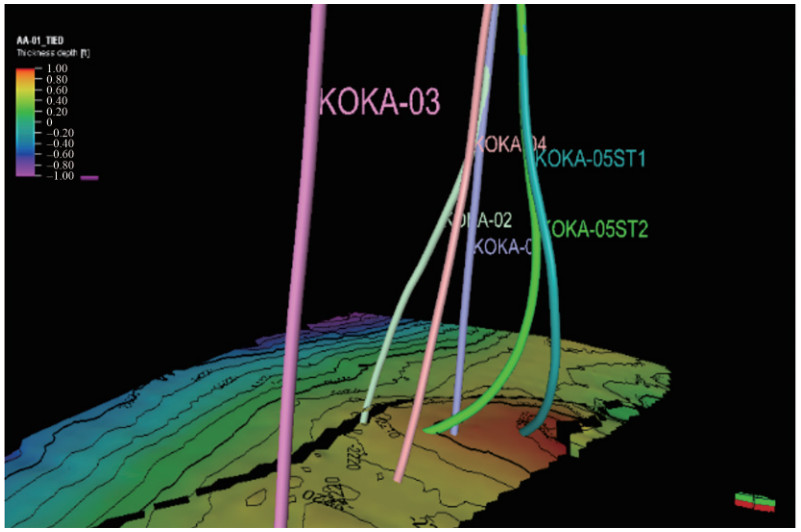 Figure 7 Static model showing six wells lacking well tops
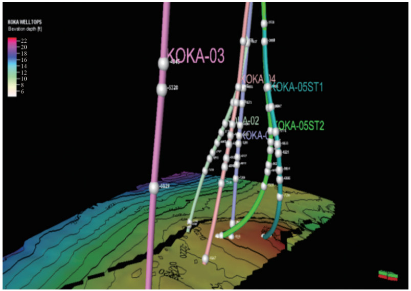 Figure 8 Static model showing six wells containing well tops and logs
2) Fluid parameters: The oil PVT or PVTO parameters were tabulated, including GOR (MSCF/STB), pressure (psi), oil formation volume factor, Bo (RB/STB), and oil viscosity (cP). The formation volume factor Bo decreases with increasing pressure up to the initial reservoir pressure of 4 056 psi at specified GOR values, while oil viscosity Cp increases with increasing pressure up to the initial reservoir pressure up to the same level (Figure 9). Similarly, the gas PVT or PVTG parameters were included but without GOR. These values were loaded into Petrel, and the quality was checked. The FVF (Bo) and cP (V) plots for the live oil PVT properties demonstrated similar trends to the plots for the dry gas PVT properties (Figure 10). The software has built-in capability to confirm data validity. For example, it will warn the user if the parameters are not decreasing in the right order. Finally, the data was plotted and viewed to confirm accuracy.
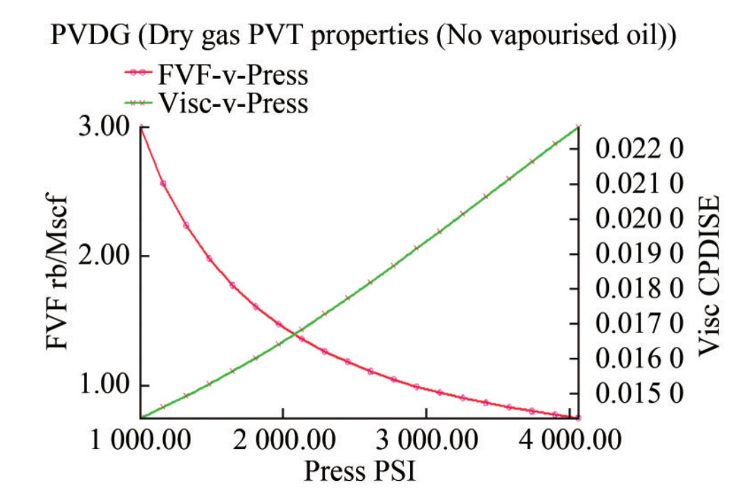 Figure 9 Dry Gas PVT properties with no vaporized oil
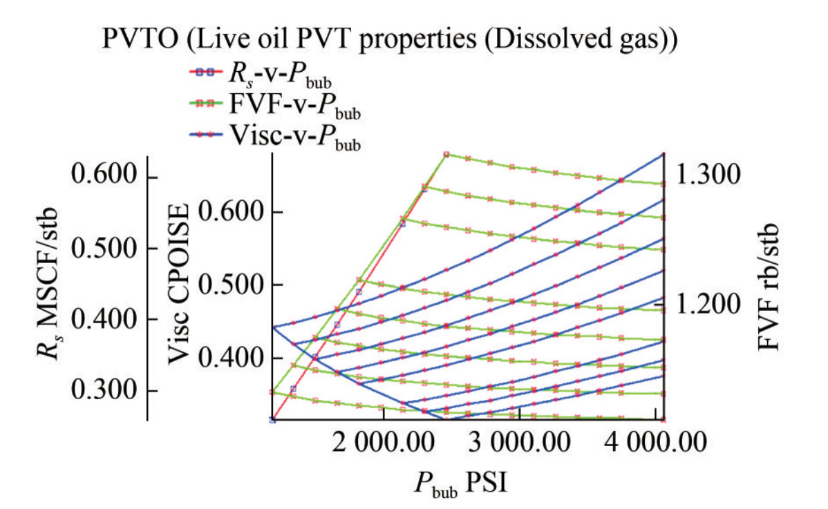 Figure 10 Live oil PVT properties with dissolved gas
3) Well data: Six wells supplied as Koka-01, Koka-02, Koka-03, Koka-04, Koka-05ST1, and Koka-05ST2, were successfully loaded into Petrel and inspected.
4) Contacts: OWC and oil up to were identified at 9 413 ft and 9 242 ft, respectively. The OWC was added as an initial condition at a datum of 6 500 ft. Since the GOC was not supplied, it was estimated and set at 6 500 ft during initialization, following the recommendation of the Petrel software.
5) SCAL/Pc: Relative permeability data was provided in various classes matching six groups of porosities ranging from 0.11 to 0.27, with a mean of 0.21. Each class contained 30 rows of data. These groups are useful for endpoint scaling, which assigns saturation functions to different regions. For this task, only class 6 data were loaded and plotted in Petrel and confirmed to be accurate at this stage.
In this case, the plots show that the nonwetting phase relative permeability curve is "S"-shaped, with the nonwetting phase starting to flow at the comparatively low saturation (Figure 11). By contrast, the wetting phase's comparative permeability curve is concave upward, starting to flow at a comparatively high saturation (Figure 12). However, relative permeability functions are complex entities and often require iterative modifications to match desired results during engineering simulations. In this regard, a correlation with the appropriate equation in the Petrel software may be required to produce values for relative permeability for the simulation process.
 Figure 11 Relative permeability curve (Gas/oil saturation functions)
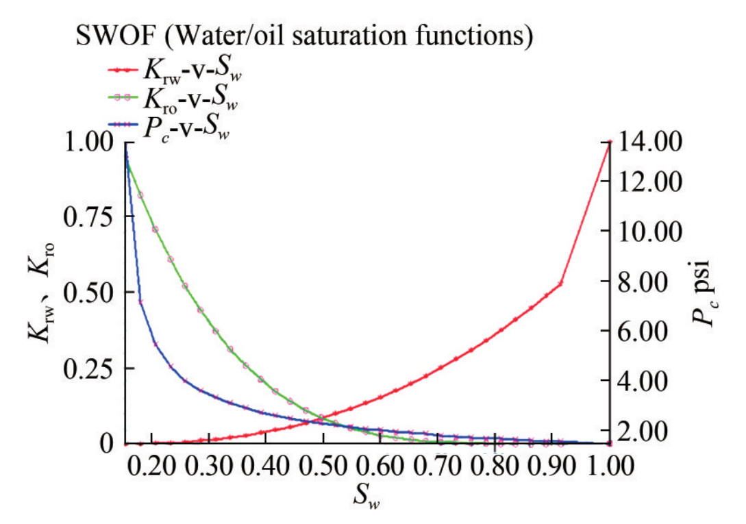 Figure 12 Relative permeability curve (Water/oil saturation functions)
6) Other data: Other quality-checked data included the initial pressure, which was used as reference pressure for the PVT properties and initial reservoir contacts.
The reservoir under study is named AA-01. At this stage, the production history data has not been loaded or confirmed.
7) Initialization: To validate our data further and set a standard background for future simulations, the reservoir was initialized using equilibration to determine its initial conditions and ensure hydrostatic equilibrium before the start of the simulation. The time-dependent properties that were defined include pressure (P), phase saturations (Sw, So, Sg), and solution gas-oil ratio (Rs). The initialization started with black oil initialization, followed by component model initialization.
During this process, no wells are required as the simulation proceeds. The reservoir model was successfully initialized, and it was noted that all fluid properties were at static equilibrium, indicated by an oil mobility ratio of zero. (Figure 13). The simulation also provided initial estimates of the oil and gas originally in place. The final phase of the initialization process will involve compositional fluid initialization of various hydrocarbon compositions.
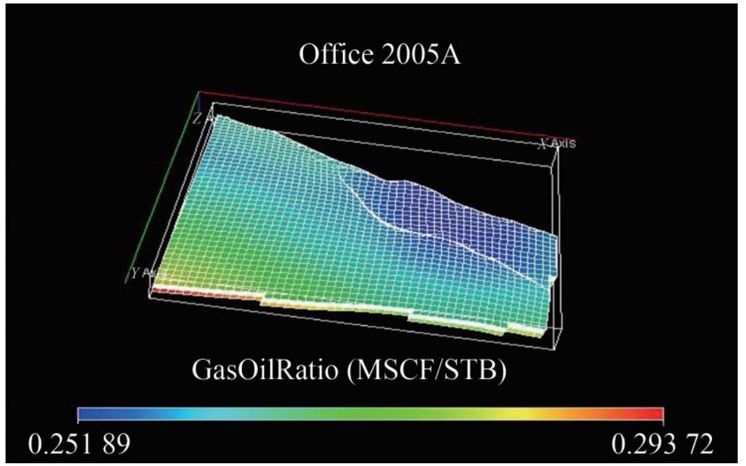 Figure 13 Initialized black oil model
Reservoir pressure and temperature conditions significantly influence the storage capacity of supercritical CO2 (Qi et al., 2010). When the supercritical condition is reached, CO2 attains a high density and gas-like viscosity, enhancing the utilization of total pore space and mobility around the reservoir (Ketzer et al., 2012). CO2 is generally stored in a supercritical phase; the density of stored CO2 was appraised at a minimum supercritical temperature (31.1 ℃) and pressure (1 070.38 psi), providing an estimate of minimum density for supercritical CO2 of 154.31 kgm-3. Literature (Hojjati et al., 2007) indicates that these values range within densities ranging from 79.08 to 996.16 kgm-3 for supercritical CO2 at supercritical temperatures and pressures.
4.2 Storage capacity and injectivity determinations for KOKA AA-01 reservoir
The geological storage prospect of the reservoir, specifically in terms of reservoir capacity and injectivity, has been quantitatively studied. To achieve this, valuable petrophysical measurements were assessed using information acquired from the well logs.
4.2.1 Reservoir capacity
The calculated porosity values of the reservoirs range from 12% to 25%, signifying that the reservoir sands are of excellent quality (Figure 14). This suggests that the reservoir has a good storage capacity for CO2 sequestration, as the sequestered CO2 is intended to replace the depleted voids in the reservoir. The available storage space in a depleted reservoir depends on the spore volume previously occupied by the produced hydrocarbon and the compaction of the pore spaces. The major lithologies encountered in the reservoir units are sand and shale, which indicates that the lithology is within the Agbada formation (Figure 19). In this study, interactive petrophysics and Microsoft Excel were used to estimate the quantity of CO2 that could be stored in the reservoirs. At the same time, some petrophysical properties were taken out from the well logs, analyzed, and quantitatively established to explain very important properties that could help assess the carbon geological storage capacity of the reservoir. According to relevant literature (Bachu et al., 2007; Ojo and Tse, 2016), parameters such as the density of the CO2 to be stored, average porosity, and water saturation of the reservoir are essential for estimating the quantity of CO2 that can be stored in a prospective geological site and for describing the promising storage site adequately.
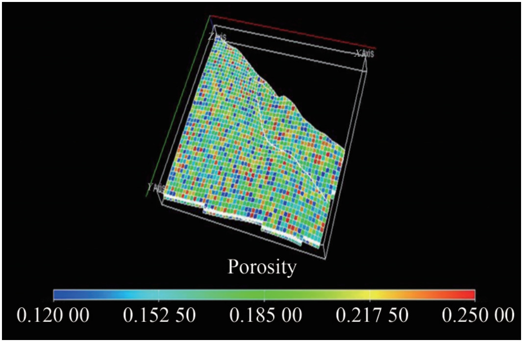 Figure 14 Porosity distribution
Geological carbon storage capacity estimates the maximum volume of CO2 that can be stored in porous media. The approaches used for estimating geological carbon storage capacities differ based on the specific set-up of the geologic formation to be utilized for storage. All methods begin with estimating the pore spaces available for CO2 injection based on established volumetric theories.
The total pore volume available for CO2 storage can be determined by assuming that all the pore space created by the produced oil and gas is filled by CO2. This is achieved by applying the following inputs:
• reservoir temperature
• the characterized PVT parameters of the reservoir fluids
• recharge to initial pressure.
This calculation provides the CO2 storage capacity, considering the overall aggregate hydrocarbon production till the end of production from the reservoir.
4.2.2 Reservoir injectivity
The estimated permeability distribution shows an average value of 1 111.0 mD for the reservoirs within the study area (Figure 15). This range of permeability value is sufficient to enhance injectivity for CO2 geological storage in the region. The entire reservoir exhibits excellent flow capability, which is crucial for a geological sequestration system to possess sufficient injectivity for the project scale. The ease with which CO2 can be injected into the reservoir is referred to as the permeability, and this permeability and thickness of storage media are connected to the injectivity (Ambrose et al., 2008). During site selection and description for CO2 geological storage, injectivity is a critical factor. It controls how fast stored CO2 is injected into the geological formation, affecting the overall cost of the storage operation by indicating that a smaller number of wells will be required for the scheme (Metz et al., 2005).
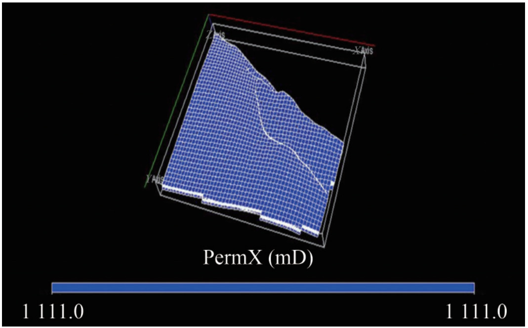 Figure 15 Permeability distribution
Reservoir pressure also plays a significant role in explaining the injectivity of the reservoir (Xie et al., 2016). The rate at which fluid is pumped in or out of a reservoir is significantly affected by reservoir pressure, as established by Birkholzer et al. (2009) and Mathias et al. (2009). By describing porosity and permeability, the injectivity of a geological formation for CO2 sequestration (Xie et al., 2016) can be sufficiently characterized. According to the International Energy Agency (2009), the reservoir in the study area possesses adequate injectivity to permit CO2 sequestration, relying on the results of this study.
4.3 Compositional simulation analysis
The compositional simulation was conducted to establish the petrophysical property variation with depth, the hydrocarbon fluid variation with depth, and the petrophysical reservoir model distribution. The parameters in Tables 3 and 4 were applied to run the compositional simulation using ECLIPSE 300.
4.3.1 Variation in fluid components with depth
The results of the simulation showing the compositional variation in hydrocarbon fluid components with depth are shown in Tables A.1 – A.3 of Appendix A. These tables indicate the composition of the hydrocarbon fluid components CO2, H2O, NaCl, and CH4 in both the oil and gas phases, as well as the total composition. The compositions of CO2, H2O, NaCl, and CH4 in oil and gas, including the total composition, are 0.000 00, 0.910 19, 0.074 0, and 0.015 00, respectively. These consistent values indicate a single phase, and the results obtained for the compositional components show that the reservoir is at static equilibrium.
4.3.2 Petrophysical properties model distribution
Applying a fully implicit simulation technique in ECLIPSE 300 generated the representative saturation table (Table A.4 in Appendix A). At static equilibrium, the representative petrophysical reservoir distribution models for the gas-oil ratio (MSCF/STB), pressure, and initialized reservoir cell structure are shown in Figures 16, 17, and 18. Determining whether the validated system-level model is suitable for its planned usage involves technical and nontechnical requirements (Thacker et al., 2004).
 Figure 16 Gas-oil ratio distribution
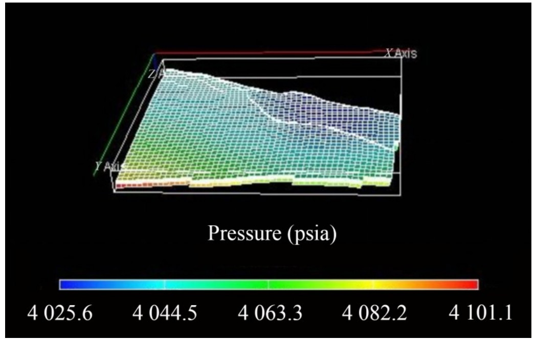 Figure 17 Pressure distribution
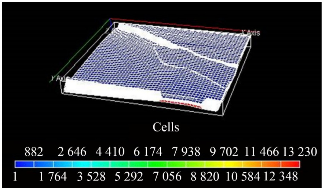 Figure 18 Initialized model
The GOR is described by the relationship GOR=Vg/Vo, where Vg and Vo represent the volumes of gas and oil produced at the surface under standard conditions. The GOR distribution, which indicates the quantity of gas ("scf ") that comes out of solution to the quantity of oil at standard conditions, is shown in Figure 16.
The compositional study results show that the GOC and water-oil contact are the same, suggesting a single-phase fluid at reservoir conditions. The fluid composition in both oil and gas phases is identical, indicating a single phase. This study also reveals a single gas phase at the reservoir conditions driven by the absence of the GOC, while the oil phase becomes evident at surface conditions. The pressure variation with reservoir depth is relatively constant under static equilibrium, with values ranging from 4 025.6 psia to 4 101.1 psia. This was an outcome of initializing the reservoir model with an undersaturated pressure of 4 056 psia.
The pressure distribution for the KOKA AA-01 reservoir is shown in Figure 17. The available PVT data combined with a comprehensible analysis of the different data types allows for a qualitative examination of reservoir fluid distribution. A two-phase region of fluid will emerge when the pressure falls below the saturation pressure, preventing the attainment of an original fluid sample. PVT parameters are essential during reservoir characterization to define the oil and gas phases. Therefore, when the formed pore volume mixture is at a single phase (either gas or oil), maximum stock tank oil (STO) recovery is achieved during production. In a two-phase mixture (i. e., cell pressure below the saturation pressure of the total mixture), PVT parameters will control the comparative motion of each phase present (from phase volume—i. e., phase saturation and viscosity), and the amount of STO transported in each phase (Baghooee et al., 2021).
The density and saturation distributions, along with the relative permeability plots at static equilibrium required before CO2 injection into the initialized reservoir for sequestration, are shown in Figures B.1 – B.7 of Appendix B, respectively. After initialization, a stability run was performed to ensure the model was thermodynamically stable. Furthermore, the model output, such as density distribution, saturation, and compositions, accurately represents the area and vertical variations across the field. The output, which represents the depth and composition variation, is then used to initialize the full field model to evaluate the field condition for CO2 sequestration (Figure 18).
The porosity distribution was reasonably good across the 3D grid, with notably good porosity distribution around Well 1 (Figure 14). In measuring total porosity, both void spaces and the whole matrix are considered, regardless of whether they are effective or ineffective. When the pore spaces are relatively connected, they are described as an effective porosity, accounting for the free-flowing fluid. The modeled porosity distribution map shows that the spatial variation in porosity values ranges between 12% and 25%, indicating that the reservoir is suitable for CO2 sequestration.
The permeability distribution model generated in this study demonstrates good lateral continuity of high permeability values within the grid block, with an average permeability value of 1 111.0 mD (Figure 15). Relative permeability is among the most valuable physical parameters for carrying out compositional simulations. The initial relative permeability curves of this reservoir flow simulation (Figure B.6 of Appendix B). This adjustment was necessary because relative permeability curves obtained from laboratory floods typically represent a much smaller scale than the drainage area of a well. Therefore, model were frequently modified during the compositional laboratory-obtained relative permeability curves often do not accurately represent multiphase flow at the reservoir scale. To address this, endpoint scaling was developed to generate relative permeability and capillary pressure curves based on a set of input curves, reducing the input data required to properly model the multiphase flow behavior and allowing adjustments to the saturation (Igwe et al., 2020). The capillary pressure curves for the KOKA AA-01 reservoir are shown in Figure B.7 of Appendix B. The average values obtained from the primary and secondary petrophysical model distributions indicate that the depleted KOKA AA-01 reservoir is a good candidate for CO2 sequestration.
4.4 Correlated KOKA AA-01 reservoir well logs
The correlated logs in Figure 19 start from the far left, or track 1, with depth measured in standard true vertical depth (SSTVD) in feet. The other tracks (from the left) include gamma-ray (GR), resistivity (RT), and density (DT). The zone of interest (pay zone) lies between horizons AA-01 at 9 250 ft and AA-01B at 9 350 ft.
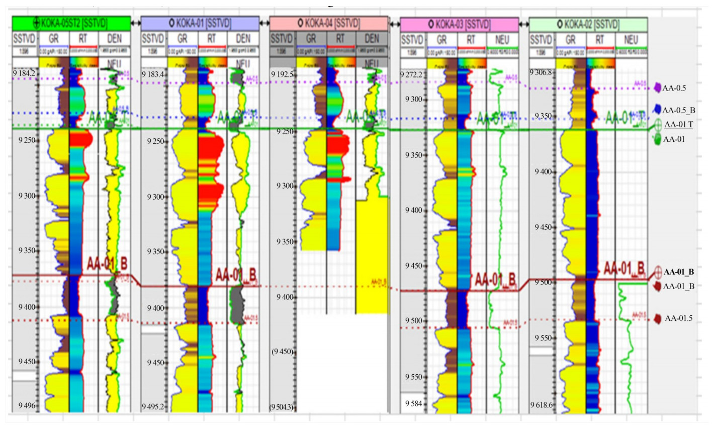 Figure 19 Correlated well logs five wells of the KOKA AA-01 reservoir
In track 2, the GR log response represents the difference between the lower GR values of sand (marked yellow) and the higher values of shale (marked brown). This GR variation is evident throughout all five wells.
Through the sandstone formation, the resistivity measurements in track 3 are color-coded: red for deep values, light blue for medium values, and deep blue for shallow values. Resistivity is notably higher in hydrocarbon zones compared to water-saturated zones in the lower part of the sand. There is a mix of medium resistivity in water-saturated zones of the sandstones across the wells and consistent shallow resistivity in the shaly formations. Wells KOKA-05ST2, KOKA-01, and KOKA-04 show the highest resistivity at the upper end of the zone of interest, while the remaining two wells (KOKA-03, KOKA-02) both indicate shallow resistivity or water-saturated zones. Neutron porosity and bulk density (last tracks) offer porosity measurements. Figure 19 Correlated well logs for five wells of the KOKA AA-01 reservoir.
Around hydrocarbon-bearing areas, the split of the curves differs based on the type of fluid encountered.
Reservoir-seal pairs are crucial for the site selection process. Reservoirs offer storage space, while seals provide vertical containment owing to their low permeability. The quality of the reservoirs and seals is evaluated by the rock type of the basin fill and its stratigraphy. The well-log correlation shows that the pay zone comprises various reservoir-seal pairs. Seal zones are characterized mainly by very low permeability shales, making them good candidates for sequestering injected CO2.
The study also confirmed the suitability of the reservoir in terms of depth, as the top of the sand is located at about 9 300 ft, which is deeper than the minimum of 2 624.67 ft, as estimated by Hasbollah and Junin (2015). The data provided for well correlation analysis utilizing gamma-ray logs and the reservoirs are laterally widespread all over the area of study with low permeable cap rock present. These factors make the study area a potential site for the geological storage of significant CO2 amounts. Studies conducted by Eigbe et al. (2023) and Yahaya-shiru et al. (2020) have shown that for large-scale CO2 underground storage to be viable, a laterally widespread reservoir and thick sealing rock must be available.
5 Conclusions
The systematic initialization procedure and associated issues advance the collaboration between static and dynamic models, aiding in modeling reservoir dynamics to achieve satisfactory simulation results for CO2 sequestration. This study set out to establish the geo-sequestration potential of depleted geologic reservoirs in the Niger Delta, focusing on reservoir capacity and injectivity. Data (well-log suits and 3D seismic data) from the depleted KOKA AA-01 reservoir have been analyzed. The estimated porosity values ranged from 12% to 25%, with an average permeability value of 1 111.0 mD. These factors contributed to determining the storage capacity and injectivity of the reservoir under investigation. The results of this study indicated that the KOKA AA-01 reservoir has sufficient storage capacity and injectivity to support CO2 sequestration effectively.
The compositional analysis of the reservoir fluid provides concise and detailed formation properties relative to depth. These plots allow interpreters to recognize different rock types, distinguish between reservoir and non-reservoir rocks, and rapidly identify pay zones in underground formations. The advantage is that the formation properties, such as porosity, permeability, pressure, and reservoir fluid saturations, can be viewed with depth. The reservoir distribution model shows that the reservoir under study has good potential for CO2 sequestration.
Furthermore, the compositional reservoir simulation captures the interplay of components and compositions within the reservoir, especially under the supercritical condition of the injected CO2. Results from this compositional analysis of the different hydrocarbon fluids (H2O, CO2, NaCl, and CH4) and the petrophysical model distribution show that the KOKA AA-01 depleted hydrocarbon reservoir is an appropriate site for CO2 storage. Key reservoir petrophysical properties such as water saturation, porosity, and density of supercritical CO2 at supercritical temperature and pressure were used to estimate the reservoir's storage capacity. The volume estimation shows that the reservoir has enough capacity to store sequestered CO2.
Additionally, a detailed well-log analysis using data from five wells in the study location estimated the top of the sand depth at 9 300 ft, which is significantly deeper than the estimated minimum value of 2 624.67 ft. This suggests that the study location has a strong potential to hold the injected CO2. However, this result was determined qualitatively. To achieve a more quantitative geologic characterization of a prospective CO2 storage site, it is necessary to adequately quantify the containment prospect of the storage location, possibly through a geo-mechanical stability analysis of CO2 storage in geologic reservoirs in the Niger Delta basin.
Nomenclature
A Area of reservoir (km2) ai, bii Correlation coefficient Bo Volume fraction of reservoir E Storage efficiency, interpolating factor ha Average thickness (km) K Permeability, K-value M Mass (megatonne) P Pressure (Pa) R Universal gas constant S Saturation T Temperature (℃) V Volume (km3) Z Compressibility factor Greek letters ϕ Porosity ϕo Average porosity ϕD Density log-derived porosity ρ Density (kgm-3) Subscripts b Bulk CO2 Carbon IV oxide c, crit Critical fl Fluid ma Matrix res Reservoir rg Relative to gas rgw Gas relative to water rh Relative to hydrocarbon rhw Hydrocarbon relative to water ro Relative to oil row Oil relative to water v Vertical w Water Swirr Irreducible water saturation Abbreviation GOC Gas–oil constant GOR Gas–oil ratio OWC Oil–water constant OGIP Original gas in place OOIP Original oil in place PVT Pressure-volume-temperature Appendix A Additional results
A.1 Variation in fluid composition with depth (Oil composition)Depth (ft) Oil composition H2O CO2 NaCl CH4 2 802.40 0.910 90 0.000 00 0.074 10 0.015 00 2 810.75 0.910 90 0.000 00 0.074 10 0.015 00 2 819.09 0.910 90 0.000 00 0.074 10 0.015 00 2 827.43 0.910 90 0.000 00 0.074 10 0.015 00 2 835.77 0.910 90 0.000 00 0.074 10 0.015 00 2 844.11 0.910 90 0.000 00 0.074 10 0.015 00 2 852.45 0.910 90 0.000 00 0.074 10 0.015 00 2 868.79 0.910 90 0.000 00 0.074 10 0.015 00 2 869.13 0.910 90 0.000 00 0.074 10 0.015 00 2 877.47 0.910 90 0.000 00 0.074 10 0.015 00 2 885.81 0.910 90 0.000 00 0.074 10 0.015 00 2 894.15 0.910 90 0.000 00 0.074 10 0.015 00 2 902.49 0.910 90 0.000 00 0.074 10 0.015 00 2 910.83 0.910 90 0.000 00 0.074 10 0.015 00 2 919.17 0.910 90 0.000 00 0.074 10 0.015 00 2 927.51 0.910 90 0.000 00 0.074 10 0.015 00 2 935.85 0.910 90 0.000 00 0.074 10 0.015 00 2 944.19 0.910 90 0.000 00 0.074 10 0.015 00 2 952.53 0.910 90 0.000 00 0.074 10 0.015 00 2 960.87 0.910 90 0.000 00 0.074 10 0.015 00 2 969.21 0.910 90 0.000 00 0.074 10 0.015 00 2 977.55 0.910 90 0.000 00 0.074 10 0.015 00 2 985.89 0.910 90 0.000 00 0.074 10 0.015 00 2 994.23 0.910 90 0.000 00 0.074 10 0.015 00 3 002.57 0.910 90 0.000 00 0.074 10 0.015 00 3 010.91 0.910 90 0.000 00 0.074 10 0.015 00 3 019.25 0.910 90 0.000 00 0.074 10 0.015 00 3 027.59 0.910 90 0.000 00 0.074 10 0.015 00 3 035.93 0.910 90 0.000 00 0.074 10 0.015 00 3 044.28 0.910 90 0.000 00 0.074 10 0.015 00 A.2 Variation in fluid composition with depth (Gas composition)Depth (ft) Gas composition H2O CO2 NACL CH4 2 802.40 0.910 90 0.000 00 0.074 10 0.015 00 2 810.75 0.910 90 0.000 00 0.074 10 0.015 00 2 819.09 0.910 90 0.000 00 0.074 10 0.015 00 2 827.43 0.910 90 0.000 00 0.074 10 0.015 00 2 835.77 0.910 90 0.000 00 0.074 10 0.015 00 2 844.11 0.910 90 0.000 00 0.074 10 0.015 00 2 852.45 0.910 90 0.000 00 0.074 10 0.015 00 2 560.79 0.910 90 0.000 00 0.074 10 0.015 00 2 569.13 0.910 90 0.000 00 0.074 10 0.015 00 2 877.47 0.910 90 0.000 00 0.074 10 0.015 00 2 585.81 0.910 90 0.000 00 0.074 10 0.015 00 2 894.15 0.910 90 0.000 00 0.074 10 0.015 00 2 902.49 0.910 90 0.000 00 0.074 10 0.015 00 2 910.83 0.910 90 0.000 00 0.074 10 0.015 00 2 919.17 0.910 90 0.000 00 0.074 10 0.015 00 2 927.51 0.910 90 0.000 00 0.074 10 0.015 00 2 935.85 0.910 98 0.000 00 0.074 10 0.015 00 2 944.19 0.910 90 0.000 00 0.074 10 0.015 00 2 952.53 0.910 90 0.000 00 0.074 10 0.015 00 2 960.87 0.910 90 0.000 00 0.074 10 0.015 00 2 969.21 0.918 90 0.000 00 0.074 10 0.015 00 2 977.55 0.910 90 0.000 00 0.074 10 0.015 00 2 985.89 0.910 90 0.000 00 0.074 10 0.015 00 2 994.23 0.910 90 0.000 00 0.074 10 0.015 00 3 002.57 0.910 90 0.000 00 0.074 10 0.015 00 3 010.91 0.910 90 0.000 00 0.074 10 0.015 00 3 177.72 0.910 90 0.000 00 0.874 10 0.015 00 3 186.06 0.910 90 0.000 00 0.074 10 0.015 00 3 194.40 0.910 90 0.000 00 0.074 10 0.015 00 3 202.74 0.910 90 0.000 00 0.074 10 0.015 00 3 211.08 0.910 90 0.000 00 0.074 10 0.015 00 A.3 Variation in fluid composition with depth (Total composition)Depth (ft) Total composition H2O CO2 Nacl CH4 2 002.40 0.910 90 0.000 00 0.074 10 0.015 00 2 010.75 0.910 20 0.000 00 0.074 10 0.015 00 2 019.09 0.910 90 0.000 00 0.074 10 0.015 00 2 027.43 0.910 90 0.000 00 0.074 10 0.015 00 2 035.77 0.910 00 0.000 00 0.074 10 0.015 00 2 844.31 0.910 90 0.000 00 0.074 10 0.015 00 2 052.45 0.910 90 0.000 00 0.074 10 0.015 00 2 860.79 0.910 90 0.000 00 0.074 10 0.015 00 2 869.13 0.910 90 0.000 00 0.074 10 0.015 00 2 077.47 0.910 20 0.000 00 0.074 10 0.015 00 2 085.81 0.910 90 0.000 00 0.074 10 0.015 00 2 094.15 0.910 90 0.000 00 0.074 10 0.015 00 2 902.49 0.910 90 0.000 00 0.074 10 0.015 00 2 919.17 0.910 90 0.000 00 0.074 10 0.015 00 2 927.51 0.910 90 0.000 00 0.074 10 0.015 00 2 935.85 0.910 90 0.000 00 0.074 10 0.015 00 2 544.19 0.910 90 0.000 00 0.074 10 0.015 00 2 952.53 0.910 90 0.000 00 0.074 10 0.015 00 2 960.10 0.910 90 0.000 00 0.074 10 0.015 00 2 969.21 0.910 90 0.000 00 0.074 10 0.015 00 2 977.55 0.910 90 0.000 00 0.074 10 0.015 00 2 985.59 0.910 90 0.000 00 0.074 10 0.015 00 2 994.23 0.910 90 0.000 00 0.074 10 0.015 00 3 002.57 0.910 90 0.000 00 0.074 10 0.015 00 3 010.91 0.910 90 0.000 00 0.074 10 0.015 00 3 019.25 0.910 90 0.000 00 0.074 10 0.015 00 3 027.59 0.910 90 0.000 00 0.074 10 0.015 00 3 194.40 0.910 90 0.000 00 0.074 10 0.015 00 3 202.74 0.910 90 0.000 00 0.074 10 0.015 00 3 211.04 0.910 90 0.000 00 0.074 10 0.015 00 A.4 Variation in composition with depthDepth
(ft)Poil
(psia)Pwat
(psia)Pgas
(psia)Deno
(1b/cu ft)Denw
(1b/cu ft)Deng
(1b/cu ft)Soil Swat Sgas Psat
(psia)Ps (obs)
(psia)2 802.40 3 904.397 2 440.798 4 025.497 28.715 63.051 28.715 4 0.000 0 0.153 0 0.847 0 0.00 0.00 2 810.75 3 906.016 2 444.434 4 027.161 28.726 63.051 28.725 8 0.000 0 0.153 0 0.847 0 0.00 0.00 2 819.09 3 907.636 2 448.070 4 028.825 28.736 63.052 28.736 2 0.000 0 0.153 0 0.847 0 0.00 0.00 2 827.43 3 909.256 2 451.707 4 030.489 28.747 63.052 28.746 6 0.000 0 0.153 0 0.847 0 0.00 0.00 2 835.77 3 910.877 2 455.343 4 032.155 28.757 63.052 28.757 0 0.000 0 0.153 0 0.847 0 0.00 0.00 2 844.11 3 912.499 2 458.979 4 033.821 28.767 63.052 28.767 4 0.000 0 0.153 0 0.847 0 0.00 0.00 2 852.45 3 914.121 2 462.615 4 035.487 28.778 63.053 28.777 7 0.000 0 0.153 0 0.847 0 0.00 0.00 2 860.79 3 915.743 2 466.252 4 037.154 28.788 63.053 28.788 1 0.000 0 0.153 0 0.847 0 0.00 0.00 2 869.13 3 917.367 2 469.888 4 038.822 28.799 63.053 28.798 5 0.000 0 0.153 0 0.847 0 0.00 0.00 2 877.47 3 918.991 2 473.525 4 040.490 28.809 63.054 28.808 9 0.000 0 0.153 0 0.847 0 0.00 0.00 2 885.81 3 920.615 2 477.161 4 042.159 28.819 63.054 28.819 3 0.000 0 0.153 0 0.847 0 0.00 0.00 2 894.15 3 922.240 2 480.798 4 043.828 28.830 63.054 28.829 7 0.000 0 0.153 0 0.847 0 0.00 0.00 2 902.49 3 923.866 2 484.434 4 045.499 28.840 63.054 28.840 1 0.000 0 0.153 0 0.847 0 0.00 0.00 2 910.83 3 925.492 2 488.071 4 047.169 28.850 63.055 28.850 5 0.000 0 0.153 0 0.847 0 0.00 0.00 2 919.17 3 927.119 2 491.707 4 048.841 28.861 63.055 28.860 9 0.000 0 0.153 0 0.847 0 0.00 0.00 2 927.51 3 928.747 2 495.344 4 050.512 28.871 63.055 28.871 2 0.000 0 0.153 0 0.847 0 0.00 0.00 2 935.85 3 930.375 2 498.981 4 052.185 28.882 63.056 28.881 6 0.000 0 0.153 0 0.847 0 0.00 0.00 2 944.19 3 932.004 2 502.618 4 053.858 28.892 63.056 28.892 0 0.000 0 0.153 0 0.847 0 0.00 0.00 2 952.53 3 933.633 2 503.254 4 055.532 28.902 63.056 28.902 4 0.000 0 0.153 0 0.847 0 0.00 0.00 Appendix B Petrophysical parameter distribution
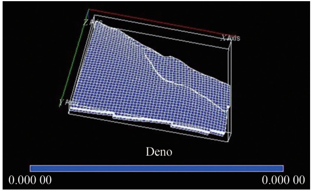 B.1 Density distribution for oil
 B.2 Density distribution for gas
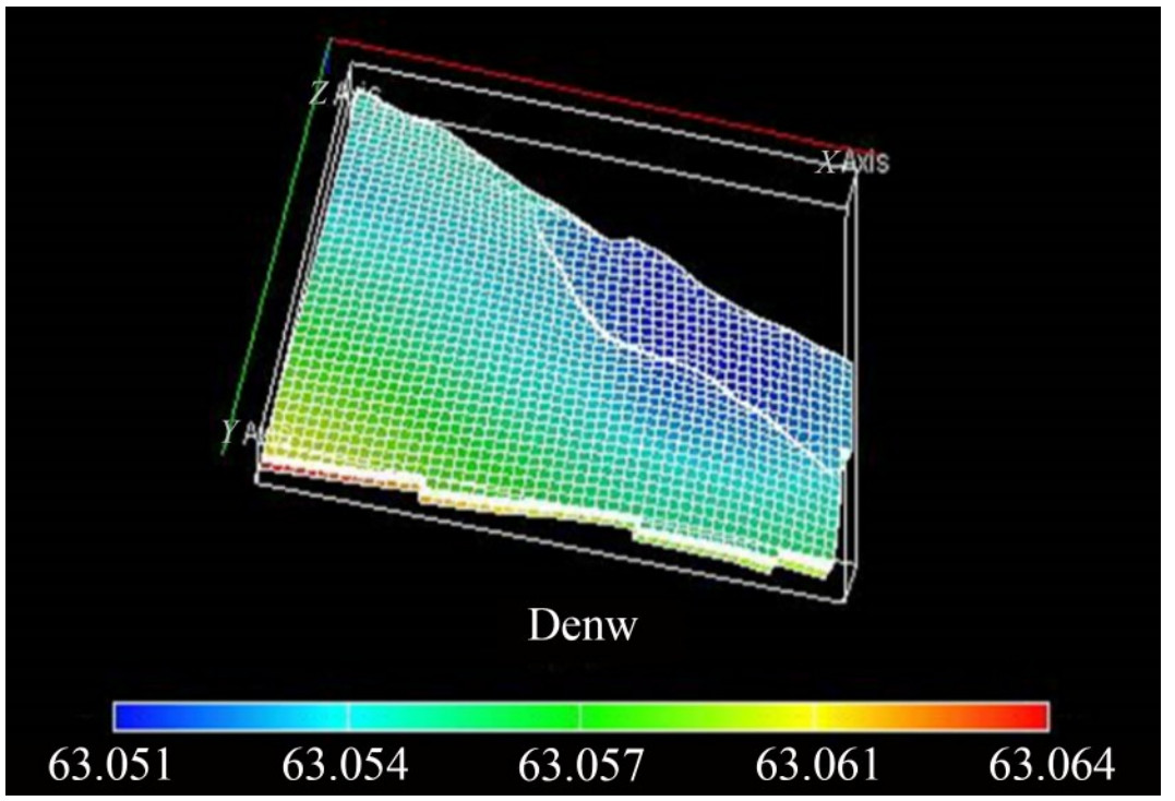 B.3 Density distribution for water
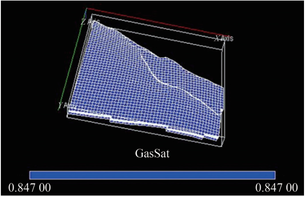 B.4 Gas saturation distribution
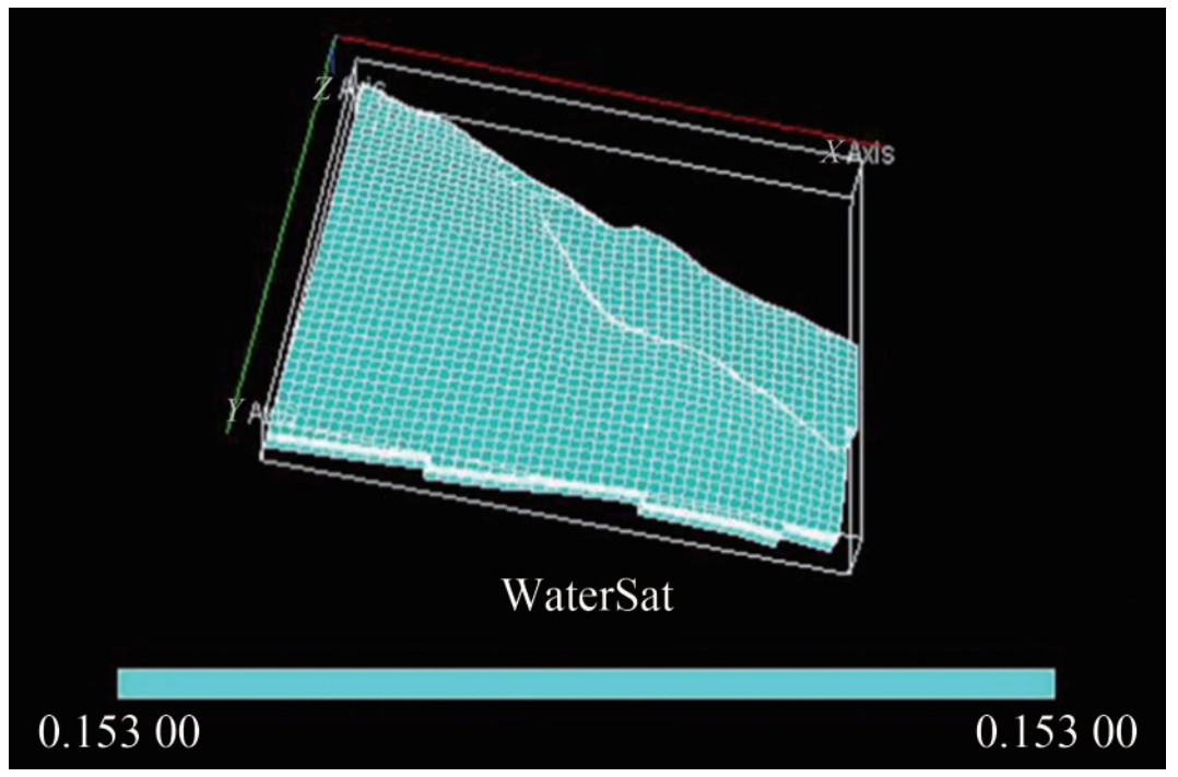 B.5 Water saturation distribution
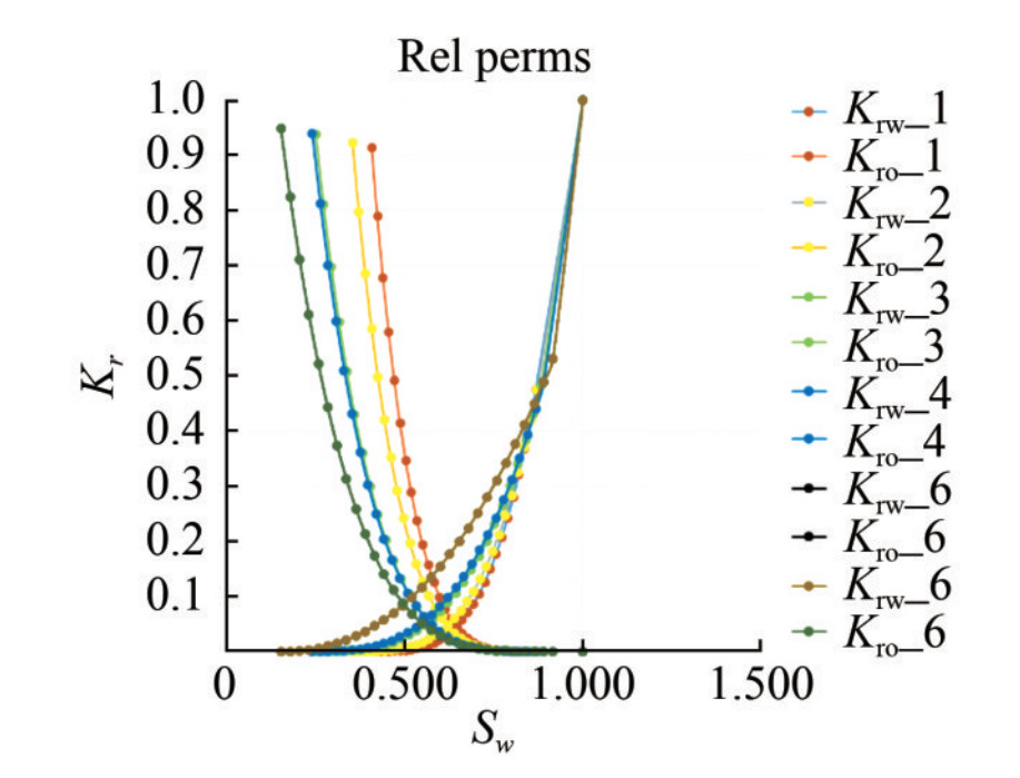 B.6 Relation permeability curvesAcknowledgement: We acknowledge the support of the Nigeria Upstream Petroleum Regulatory Commission (NUPRC) and Seplat Petroleum Development Company for the supply of the data used for this study.
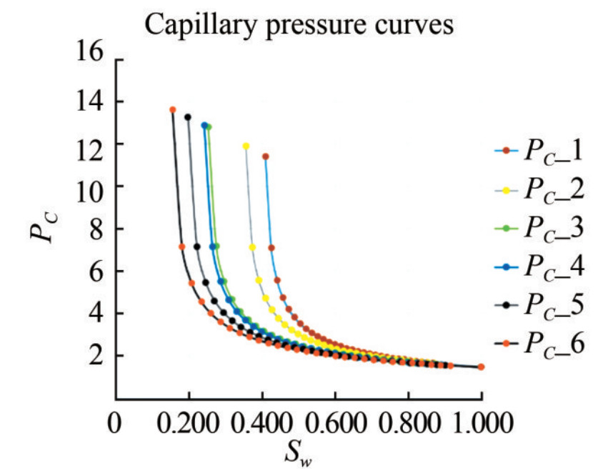 B.7 Capillary pressure curvesCompeting interestThe authors have no competing interests to declare that are relevant to the content of this article.
 -
Figure 1 Carbon capture, use, and storage supply chain (Source: Rocky Mountain Coal Mining Institute. Atlas iv, 2012)
Figure 2 Carbon dioxide storage options (Orr, 2009)
Figure 3 Geological map showing the Niger Delta and environs (Whiteman, 1982)
Figure 4 Stratigraphic column of the Niger Delta basin. Modified from Doust and Omatsola (1990)
Figure 5 Phase diagram matching the initial conditions of fluid in PVTi
Figure 6 Effect of gas injection
Figure 7 Static model showing six wells lacking well tops
Figure 8 Static model showing six wells containing well tops and logs
Figure 9 Dry Gas PVT properties with no vaporized oil
Figure 10 Live oil PVT properties with dissolved gas
Figure 11 Relative permeability curve (Gas/oil saturation functions)
Figure 12 Relative permeability curve (Water/oil saturation functions)
Figure 13 Initialized black oil model
Figure 14 Porosity distribution
Figure 15 Permeability distribution
Figure 16 Gas-oil ratio distribution
Figure 17 Pressure distribution
Figure 18 Initialized model
Figure 19 Correlated well logs five wells of the KOKA AA-01 reservoir
B.1 Density distribution for oil
B.2 Density distribution for gas
B.3 Density distribution for water
B.4 Gas saturation distribution
B.5 Water saturation distribution
B.6 Relation permeability curves
B.7 Capillary pressure curves
Table 1 Primary and secondary variables with phase changes
S/N Phase state Present component Primary variables Secondary variables (Phase vhanges) Oil phase appearance Gas phase appearance Brine phase appearance 1 All 3 Phases (Oil, Gas and Brine) O, W, CO2, CH4 P, T, Sw, p_i, µ_i, B_i, cp_i, k_i K_i, ϕ_i, ∇P, ∇T nil nil nil 2 2 Phases (Brine and Gas) W, CO2, CH4 P, T, Sw, p_i, µ_i, B_i, cp_i, k_i nil x_gas>0
$X_b^g \geqslant\left(X_b^g\right) \max$X_brine>0
$X_g^b \geqslant\left(X_g^b\right) \max$3 2 Phases (Oil and Brine) O, W P, T, Sw, p_i, µ_i, B_i, cp_i, k_i x_oil>0
$X_b^o \geqslant\left(X_b^o\right) \max$nil X_brine>0
$X_o^b \geqslant\left(X_o^b\right) \max$4 2 Phases (Oil and Gas) O P, T, Sw, p_i, µ_i, B_i, cp_i, k_i x_oil>0
$X_g^o \geqslant\left(X_g^o\right) \max$x_gas>0
$X_o^g \geqslant\left(X_o^g\right) \max$nil 5 Brine Phase W P, T, Sw, p_i, µ_i, B_i, cp_i, k_i nil nil $\mathrm{x}_{\mathrm{gas}}<0>\mathrm{x}_{\text {_oil }} \\ \text { X_brine }>0$ 6 Oil Rich Phase O P, T, S, p_i, µ_i, B_i, cp_i, k_i xgas<0>x_brine
x_oil>0nil nil 7 Gas Rich Phase CO2, CH4 P, T, S, p_i, µ_i, B_i, cp_i, k_i nil xoil<0>x_brine
x_gas>0nil Table 2 List of data and validation procedures
S/N File Remark Format Parent folder Provided as Validation 1 Static Model The entire geologic model can help confirm the given input data in PETREL. PG 1. KOKA Petrel Project.ptd
2. KOKA Petrel Project.petWas loaded into Petrel and model confirmed. 2 GRID The ASCII format is preferable ASCII (*GRDE CL) and BINARY (*GRID, *EGRID) formats. Same as 1 above Same as 1 above Same as 1 above 3 PVT Data Reservoir Formation Test if available will suffice PDF or EXCEL RE KOKA.PVT.xlsx 1. Conclusively validated by Model Initialization
2 Indicates crude is undersaturated Oil
3 Indicates Initial Pressure, Pi@4056 psia4 Well Data Well Logs, etc ASCII or EXCEL PP Koka-001.asc, Koka-002.asc, Koka-003.asc, Koka-004.asc, Koka-005.asc, Loaded in a separated model and still confirmed in the given static model 5 Contacts OWC/GOC logged from respective wells ASCII or EXCEL PP Koka Reservoir Average.xlsx To be loaded in PETREL, and ECLIPSE as a final confirmation 6 SCAL Data Relative Permeability and Capillary Pressure Any of ASCII, EXCEL, and PDF RE 1 Koka_SCAL_Kr_PC.xlsx Loaded in PETREL, and ECLIPSE as and confirm to have different classes of Rel Perm endpoint for Oil/Water. 7 Initial Pressure/Pressure Data RE KOKA.PVT.xlsx, Koka_Production_Pressure.xlsx Validated during initialization in Petrel and Eclipse 8 Production History Data Example, 30 years of Oil and Gas production up to depleted (mature stage). With/Without CO2 Recovery. ASCII or EXCEL PT Koka_Production_Pressure.xls/Koka Well Production To be loaded in PETREL and ECLIPSE as a final confirmation. Table 3 Reservoir parameters
Parameter Value Initial reservoir pressure (psia) 4 056 Reservoir temperature (°F) 177 Range of porosity values 0.11–0.27 Mean porosity 0.21 Average permeability value (mD) 1 111.0 Maximum number of wells 0 Maximum number of separators 5 Grid dimension (ft3) 50×42×63 Total grids cells 132 300 Reservoir crest (ftss) 9 238 OWC (fts) 9 314 Hydrocarbon column (ftss) 76 Table 4 Initialized volume of reservoir fluids
Fluid Component Value Oil (Res Vol) (fb) 0 Water (Res Vol) (rb) 9 374 013.1 Gas (Res Vol) (rb) 51 854 046 Water (Surf Vol) (stb) 9 477 775.2 Oil (wrt separator) (stb) 1.897 465 2×10⁸ Gas (wrt separator) (Mscf) 0 Table 5 Value of bif coefficients in Equation (5) for pressures below 3 000 psi (Ouyang, 2011)
i bi0 bi1 bi2 bi3 bi4 0 -2.15×10⁵ 1.17×10⁴ -2.30×10² 1.97 -6.18×10² 1 4.76×10² -2.62×101 5.22×10⁻¹ -4.49×10⁻³ 1.42×10⁻⁵ 2 -3.71×10⁻¹ 2.07×10⁻² -4.17×10⁻⁴ 3.62×10⁻⁶ -1.16×10⁻⁸ 3 1.23×10⁻⁴ -6.3×10⁻⁶ 1.41×10⁻⁷ -1.23×10⁻⁹ 3.95×10⁻¹² 4 -1.47×10⁻⁸ -8.34×10⁻¹⁰ -1.70×10⁻¹¹ 1.50×10⁻¹³ -4.84×10⁻¹⁶ A Area of reservoir (km2) ai, bii Correlation coefficient Bo Volume fraction of reservoir E Storage efficiency, interpolating factor ha Average thickness (km) K Permeability, K-value M Mass (megatonne) P Pressure (Pa) R Universal gas constant S Saturation T Temperature (℃) V Volume (km3) Z Compressibility factor Greek letters ϕ Porosity ϕo Average porosity ϕD Density log-derived porosity ρ Density (kgm-3) Subscripts b Bulk CO2 Carbon IV oxide c, crit Critical fl Fluid ma Matrix res Reservoir rg Relative to gas rgw Gas relative to water rh Relative to hydrocarbon rhw Hydrocarbon relative to water ro Relative to oil row Oil relative to water v Vertical w Water Swirr Irreducible water saturation Abbreviation GOC Gas–oil constant GOR Gas–oil ratio OWC Oil–water constant OGIP Original gas in place OOIP Original oil in place PVT Pressure-volume-temperature A.1 Variation in fluid composition with depth (Oil composition)
Depth (ft) Oil composition H2O CO2 NaCl CH4 2 802.40 0.910 90 0.000 00 0.074 10 0.015 00 2 810.75 0.910 90 0.000 00 0.074 10 0.015 00 2 819.09 0.910 90 0.000 00 0.074 10 0.015 00 2 827.43 0.910 90 0.000 00 0.074 10 0.015 00 2 835.77 0.910 90 0.000 00 0.074 10 0.015 00 2 844.11 0.910 90 0.000 00 0.074 10 0.015 00 2 852.45 0.910 90 0.000 00 0.074 10 0.015 00 2 868.79 0.910 90 0.000 00 0.074 10 0.015 00 2 869.13 0.910 90 0.000 00 0.074 10 0.015 00 2 877.47 0.910 90 0.000 00 0.074 10 0.015 00 2 885.81 0.910 90 0.000 00 0.074 10 0.015 00 2 894.15 0.910 90 0.000 00 0.074 10 0.015 00 2 902.49 0.910 90 0.000 00 0.074 10 0.015 00 2 910.83 0.910 90 0.000 00 0.074 10 0.015 00 2 919.17 0.910 90 0.000 00 0.074 10 0.015 00 2 927.51 0.910 90 0.000 00 0.074 10 0.015 00 2 935.85 0.910 90 0.000 00 0.074 10 0.015 00 2 944.19 0.910 90 0.000 00 0.074 10 0.015 00 2 952.53 0.910 90 0.000 00 0.074 10 0.015 00 2 960.87 0.910 90 0.000 00 0.074 10 0.015 00 2 969.21 0.910 90 0.000 00 0.074 10 0.015 00 2 977.55 0.910 90 0.000 00 0.074 10 0.015 00 2 985.89 0.910 90 0.000 00 0.074 10 0.015 00 2 994.23 0.910 90 0.000 00 0.074 10 0.015 00 3 002.57 0.910 90 0.000 00 0.074 10 0.015 00 3 010.91 0.910 90 0.000 00 0.074 10 0.015 00 3 019.25 0.910 90 0.000 00 0.074 10 0.015 00 3 027.59 0.910 90 0.000 00 0.074 10 0.015 00 3 035.93 0.910 90 0.000 00 0.074 10 0.015 00 3 044.28 0.910 90 0.000 00 0.074 10 0.015 00 A.2 Variation in fluid composition with depth (Gas composition)
Depth (ft) Gas composition H2O CO2 NACL CH4 2 802.40 0.910 90 0.000 00 0.074 10 0.015 00 2 810.75 0.910 90 0.000 00 0.074 10 0.015 00 2 819.09 0.910 90 0.000 00 0.074 10 0.015 00 2 827.43 0.910 90 0.000 00 0.074 10 0.015 00 2 835.77 0.910 90 0.000 00 0.074 10 0.015 00 2 844.11 0.910 90 0.000 00 0.074 10 0.015 00 2 852.45 0.910 90 0.000 00 0.074 10 0.015 00 2 560.79 0.910 90 0.000 00 0.074 10 0.015 00 2 569.13 0.910 90 0.000 00 0.074 10 0.015 00 2 877.47 0.910 90 0.000 00 0.074 10 0.015 00 2 585.81 0.910 90 0.000 00 0.074 10 0.015 00 2 894.15 0.910 90 0.000 00 0.074 10 0.015 00 2 902.49 0.910 90 0.000 00 0.074 10 0.015 00 2 910.83 0.910 90 0.000 00 0.074 10 0.015 00 2 919.17 0.910 90 0.000 00 0.074 10 0.015 00 2 927.51 0.910 90 0.000 00 0.074 10 0.015 00 2 935.85 0.910 98 0.000 00 0.074 10 0.015 00 2 944.19 0.910 90 0.000 00 0.074 10 0.015 00 2 952.53 0.910 90 0.000 00 0.074 10 0.015 00 2 960.87 0.910 90 0.000 00 0.074 10 0.015 00 2 969.21 0.918 90 0.000 00 0.074 10 0.015 00 2 977.55 0.910 90 0.000 00 0.074 10 0.015 00 2 985.89 0.910 90 0.000 00 0.074 10 0.015 00 2 994.23 0.910 90 0.000 00 0.074 10 0.015 00 3 002.57 0.910 90 0.000 00 0.074 10 0.015 00 3 010.91 0.910 90 0.000 00 0.074 10 0.015 00 3 177.72 0.910 90 0.000 00 0.874 10 0.015 00 3 186.06 0.910 90 0.000 00 0.074 10 0.015 00 3 194.40 0.910 90 0.000 00 0.074 10 0.015 00 3 202.74 0.910 90 0.000 00 0.074 10 0.015 00 3 211.08 0.910 90 0.000 00 0.074 10 0.015 00 A.3 Variation in fluid composition with depth (Total composition)
Depth (ft) Total composition H2O CO2 Nacl CH4 2 002.40 0.910 90 0.000 00 0.074 10 0.015 00 2 010.75 0.910 20 0.000 00 0.074 10 0.015 00 2 019.09 0.910 90 0.000 00 0.074 10 0.015 00 2 027.43 0.910 90 0.000 00 0.074 10 0.015 00 2 035.77 0.910 00 0.000 00 0.074 10 0.015 00 2 844.31 0.910 90 0.000 00 0.074 10 0.015 00 2 052.45 0.910 90 0.000 00 0.074 10 0.015 00 2 860.79 0.910 90 0.000 00 0.074 10 0.015 00 2 869.13 0.910 90 0.000 00 0.074 10 0.015 00 2 077.47 0.910 20 0.000 00 0.074 10 0.015 00 2 085.81 0.910 90 0.000 00 0.074 10 0.015 00 2 094.15 0.910 90 0.000 00 0.074 10 0.015 00 2 902.49 0.910 90 0.000 00 0.074 10 0.015 00 2 919.17 0.910 90 0.000 00 0.074 10 0.015 00 2 927.51 0.910 90 0.000 00 0.074 10 0.015 00 2 935.85 0.910 90 0.000 00 0.074 10 0.015 00 2 544.19 0.910 90 0.000 00 0.074 10 0.015 00 2 952.53 0.910 90 0.000 00 0.074 10 0.015 00 2 960.10 0.910 90 0.000 00 0.074 10 0.015 00 2 969.21 0.910 90 0.000 00 0.074 10 0.015 00 2 977.55 0.910 90 0.000 00 0.074 10 0.015 00 2 985.59 0.910 90 0.000 00 0.074 10 0.015 00 2 994.23 0.910 90 0.000 00 0.074 10 0.015 00 3 002.57 0.910 90 0.000 00 0.074 10 0.015 00 3 010.91 0.910 90 0.000 00 0.074 10 0.015 00 3 019.25 0.910 90 0.000 00 0.074 10 0.015 00 3 027.59 0.910 90 0.000 00 0.074 10 0.015 00 3 194.40 0.910 90 0.000 00 0.074 10 0.015 00 3 202.74 0.910 90 0.000 00 0.074 10 0.015 00 3 211.04 0.910 90 0.000 00 0.074 10 0.015 00 A.4 Variation in composition with depth
Depth
(ft)Poil
(psia)Pwat
(psia)Pgas
(psia)Deno
(1b/cu ft)Denw
(1b/cu ft)Deng
(1b/cu ft)Soil Swat Sgas Psat
(psia)Ps (obs)
(psia)2 802.40 3 904.397 2 440.798 4 025.497 28.715 63.051 28.715 4 0.000 0 0.153 0 0.847 0 0.00 0.00 2 810.75 3 906.016 2 444.434 4 027.161 28.726 63.051 28.725 8 0.000 0 0.153 0 0.847 0 0.00 0.00 2 819.09 3 907.636 2 448.070 4 028.825 28.736 63.052 28.736 2 0.000 0 0.153 0 0.847 0 0.00 0.00 2 827.43 3 909.256 2 451.707 4 030.489 28.747 63.052 28.746 6 0.000 0 0.153 0 0.847 0 0.00 0.00 2 835.77 3 910.877 2 455.343 4 032.155 28.757 63.052 28.757 0 0.000 0 0.153 0 0.847 0 0.00 0.00 2 844.11 3 912.499 2 458.979 4 033.821 28.767 63.052 28.767 4 0.000 0 0.153 0 0.847 0 0.00 0.00 2 852.45 3 914.121 2 462.615 4 035.487 28.778 63.053 28.777 7 0.000 0 0.153 0 0.847 0 0.00 0.00 2 860.79 3 915.743 2 466.252 4 037.154 28.788 63.053 28.788 1 0.000 0 0.153 0 0.847 0 0.00 0.00 2 869.13 3 917.367 2 469.888 4 038.822 28.799 63.053 28.798 5 0.000 0 0.153 0 0.847 0 0.00 0.00 2 877.47 3 918.991 2 473.525 4 040.490 28.809 63.054 28.808 9 0.000 0 0.153 0 0.847 0 0.00 0.00 2 885.81 3 920.615 2 477.161 4 042.159 28.819 63.054 28.819 3 0.000 0 0.153 0 0.847 0 0.00 0.00 2 894.15 3 922.240 2 480.798 4 043.828 28.830 63.054 28.829 7 0.000 0 0.153 0 0.847 0 0.00 0.00 2 902.49 3 923.866 2 484.434 4 045.499 28.840 63.054 28.840 1 0.000 0 0.153 0 0.847 0 0.00 0.00 2 910.83 3 925.492 2 488.071 4 047.169 28.850 63.055 28.850 5 0.000 0 0.153 0 0.847 0 0.00 0.00 2 919.17 3 927.119 2 491.707 4 048.841 28.861 63.055 28.860 9 0.000 0 0.153 0 0.847 0 0.00 0.00 2 927.51 3 928.747 2 495.344 4 050.512 28.871 63.055 28.871 2 0.000 0 0.153 0 0.847 0 0.00 0.00 2 935.85 3 930.375 2 498.981 4 052.185 28.882 63.056 28.881 6 0.000 0 0.153 0 0.847 0 0.00 0.00 2 944.19 3 932.004 2 502.618 4 053.858 28.892 63.056 28.892 0 0.000 0 0.153 0 0.847 0 0.00 0.00 2 952.53 3 933.633 2 503.254 4 055.532 28.902 63.056 28.902 4 0.000 0 0.153 0 0.847 0 0.00 0.00 -
Ajayi T, Gomes JS, Achinta Bera A (2019) A review of CO2 storage in geological formations emphasizing modelling, monitoring and capacity estimation approaches. Petroleum Science 16: 1028-1063. https://doi.org/10.1007/s12182-019-0340-8 Ambrose WA, Lakshminarasimhan S, Holtz MH, Núñez-López V, Hovorka SD, Duncan I (2008) Geologic Factors controlling CO2 storage capacity and permanence: Case studies based on experience with heterogeneity in oil and gas reservoirs applied to CO2 storage. Environmental Earth Science 54(8): 1619-1633 Avbovbo AA (1978) Geo-thermal gradients in the Southern Nigerian basin. Bulletin of Canadian Petroleum Geology 26(2): 268-274 Bachu S, Bonijoly D, Bradshaw J, Burruss R, Holloway S, Christensen NP (2007) CO2 storage capacity estimation: methodology and gaps. International Journal of Greenhouse Gas Control 1(4): 430-443. https://doi.org/10.1016/S1750-5836(07)00086-2 Badru L (2020) Climate change in Nigeria: Causes, effects and legal framework. Unilag Law Review 4(1): 186-203 Baghooee H (2021) Characterization of the fluid distribution in petroleum reservoirs. PhD thesis, Technical University of Denmark, Copenhagen Bahadori A, Vuthaluru HB, Mokhatab S (2009) New correlations predict aqueous solubility and density of carbon dioxide. International Journal of Greenhouse Gas Control 3(4): 474-480 https://doi.org/10.1016/j.ijggc.2009.01.003 Birkholzer JT, Zhou Q, Tsang C-F (2009) Large-scale impact of CO2 storage in deep saline aquifers: A sensitivity study on pressure response in stratified systems. International Journal of Greenhouse Gas Control 3(2): 181-194 https://doi.org/10.1016/j.ijggc.2008.08.002 Bogatyrev AF, Makeenkova OA, Nezovitina, MA (2015) Experimental study of thermal diffusion in multicomponent gaseous systems. International Journal of Thermophysics 36: 633-647 https://doi.org/10.1007/s10765-014-1818-7 Carlson MF (2006) Practical reservoir simulation: Penn Well Corporation, Tulsa, OK, USA Chang YB, Coats BK, Nolen JS (1998) A compositional model for CO2 floods including CO2 solubility in water. Paper SPE 35164, SPE Reservoir Evaluation Engineering 1(2): 155-160 https://doi.org/10.2118/35164-PA Davies OA, Davies DH, Ngeri PA (2018) Comparative analysis of porosity estimates in a sandstone reservoir: The Niger Delta as case study. Journal of Science and Engineering Research 5(11): 102-111 Doust H, Omatsola E (1990) Divergent/passive margin basins. Bullettin of American Association of Petroleum Geologists Memoir 48: 201-238. https://10.1306/m48508c4 Eigbe PA, Ajayi OO, Olakoyejo OT, Fadipe OL, Efe S, Adelaja AO (2022). A review of CO2 sequestration in underground geological formations: recent developments and potential opportunities in the Niger Delta. In: Urban Energy Systems towards Carbon Neutrality. Energy Proceedings: 1-10. https://doi.org/10.46855/energy-proceedings-10340 Eigbe PA, Ajayi OO, Olakoyejo OT, Fadipe OL, Efe S, Adelaja AO (2023) A general review of CO2 sequestration in underground geological formations and assessment of depleted hydrocarbon reservoirs in the Niger Delta. Journal of Applied Energy 350: 121723 https://doi.org/10.1016/j.apenergy.2023.121723 Giwa SO, Adama OO, Akinyemi OO (2014) Baseline black carbon emissions for gas flaring in the Niger Delta region of Nigeria. Journal of Natural Gas Science and Engineering 20: 373-379 https://doi.org/10.1016/j.jngse.2014.07.026 Grobe M, Pashin JC, Dodge RL (2009) Carbon dioxide sequestration in geological media: state of the science. In: AAPG studies in geology. American Association of Petroleum Geologists 59: ISBN: 0891810668 Tulsa, OK. xi, 715. https://doi.org/10.1306/st591317 Guo G, Diaz MA, Paz F, Smalley J, Waninger EA (2007) Rock typing as an effective tool for permeability and water saturation modelling: a case study in a clastic reservoir in the Oriente Basin. SPE Reservoir Evaluation and Engineering 10(6): 730-739. DOI: 102118/97033-PA https://doi.org/ 10.2118/97033-PA Hasbollah DZA, Junin R (2015) A preliminary basin scale evaluation framework of potential sedimentary basins in Malaysia for carbon dioxide sequestration. Journal of Chemical Engineering Transactions 45: 1537-1542. DOI: 10.3303/CET1545257 Hoffert MI, Caldeira K, Benford G, Criswell DR, Green C, Herzog H, Jain AK, Kheshgri HS, Lackner KS, Lewis JS, Lightfoot HD, Manheimer W, Mankins JC, Mauel ME, Perkins LJ, Schlesinger ME, Volk T, Wigley TML (2002) Advanced technology paths to global climate stability: Energy for a greenhouse planet. Journal of Science 298: 981-987 Hojjati M, Yamini Y, Khajeh M, Vatanara A (2007) Solubility of some statin drugs in supercritical carbon dioxide and representing the solute solubility data with several density-based correlations. Journal of Supercritical Fluids 41(2): 187-194 https://doi.org/10.1016/j.supflu.2006.10.006 Hospers J (1965) Gravity field and structure of the Niger Delta, Nigeria, West Africa. Geological Society of American Bulletin 76(4): 407-422. https://doi.org/10.1130/0016-7606(1965)76[407:GFASOT]2.0.CO;2 Igwe I, Gholinezhad J, Sayed MGH, Obuagu F (2020) Technical implications of neglecting compositional grading effects in petroleum reservoir simulation models. Journal of Energy and Fuels 34(2): 1467-1481 https://doi.org/10.1021/acs.energyfuels.9b03528 International Energy Agency (2009) Development of storage coefficients for CO2 storage in deep saline formations. In International Energy Agency Greenhouse Gas Programme Report 2009/12 Ishisone M (2004) Gas flaring in the Niger Delta: The potential benefits of its reduction on the local economy and environment. Journal of Environmental Science and Economics. Corpus ID: 53686613 Jaramillo JM, Barrufet MA (2001) Effects in the determination of oil reserves due to gravitational compositional gradients in near-critical reservoirs. SPE Annual Technical Conference and Exhibition, New Orleans, Louisiana Kaplan A, Lusser CU, Norton IO (1994) Tectonic map of the world, panel 10: Tulsa, scale 1: 10 000 000. American Association of Petroleum Geologists, Tulsa Ketzer JM, Iglesias R, Einloft S (2012) Reducing greenhouse gas emissions with CO2 capture and geological storage. In: W. -Y. Chen, J. Seiner, T. Suzuki and M. Lackner (Editors), Handbook of Climate Change Mitigation. Springer US: 1405-1440 Klett TR, Ahlbrandt TS, Schmoker JW, Dolton JL (1997) Ranking of the world's oil and gas provinces by known petroleum volumes: U.S. Geological Survey Open-file Report, 97-463 Krygowski DA (2003) Guide to petrophysical interpretation. Austin Texas, 147 Kulke H. (1995) Regional Petroleum Geology of the World. Part Ⅱ: Africa, America, Australia and Antarctica: Berlin, Gebrüder Borntraeger, 143-172 Lackner KS (2003) Climate change. A guide to CO2 sequestration. Journal of Science 300: 1677-1678 Masson-Delmotte VP, Zhai P, Pirani SL, Connors C, Péan S, Berger N, Scheel Monteiro PM (2021) IPCC, 2021: Summary for policymakers. In: Climate change 2021: The physical science basis. Contribution of working group i to the sixth assessment report of the intergovernmental panel on climate change Mathias SA, Hardisty PE, Trudell MR, Zimmerman RW (2009) Screening and selection of sites for CO2 sequestration based on pressure build-up. International Journal Greenhouse Gas Control 3(5): 577-585 https://doi.org/10.1016/j.ijggc.2009.05.002 Metz B, Davidson O, DeConinck H, Loos M, Meyer L (2005) IPCC special report on carbon dioxide capture and storage. Prepared by Working Group Ⅲ of the Intergovernmental Panel on Climate Change. IPCC, Cambridge University Press, Cambridge, United Kingdom and New York Mkemai RM, Gong B (2020) Geological performance evaluation of CO2 sequestration in depleted oil reservoirs: A simulation study on the effect of water saturation and vertical to horizontal permeability ratio. Journal of Natural Gas Science and Engineering 76: 103196. https://doi.org/10.1016/j.jngse.2020.103196 National Energy Technology Laboratory (2007) Carbon sequestration atlas of the United States and Canada. US Department of Energy, Office of Fossil Energy Nikpoor MH, Kharrat R, Chen Z (2013) The modelling of 3D compositional grading and plus fraction molecular weight change in non-isothermal petroleum reservoirs. Energy Sources A: Recovery, Utilization and Environmental Effects 35(2): 99-109. DOI: 10.1080/15567036.2010.501365 OECD/ITF (2009) Reducing transport greenhouse gas emissions. Available from www.internationaltransportforum.org/Pub/pdf/10GHGTrends.pdf. Accessed on January 4, 2016 Ojo AC, Tse AC (2016) Geological characterization of depleted oil and gas reservoirs for carbon sequestration potentials in a field in the Niger Delta, Nigeria. Journal of Applied Science and Environmental Management 20(1): 45-55 Oldenburg CM, Pruess K, Benson SM (2001) Process modelling of CO2 injection into natural gas reservoirs for carbon sequestration and enhanced gas recovery. Journal of Energy and Fuel 15(2): 293-298. https://doi.org/10.1021/ef000247h Orr FM (2009) Onshore geologic storage of CO2. Journal of Science 325: 1656-1658 Oseji JO (2007) Thermal gradient in the vicinity of Kwale/Okpai gas plant, Delta state, Nigeria: Preliminary observations. Journal of Environmentalist 27: 311-314 https://doi.org/10.1007/s10669-007-9007-x Ouyang L-B (2011) New correlations for predicting the density and viscosity of supercritical carbon dioxide under conditions expected in carbon capture and sequestration operations. The Open Petroleum Engineering Journal 4: 13-21 Owolabi OO, LongJohn TF, Ajienka JA (1994) An empirical expression for permeability in unconsolidated sands of the eastern Niger Delta. Journal of Petroleum Geology 17(1): 111-116 https://doi.org/10.1111/j.1747-5457.1994.tb00117.x Pacala S, Socolow R (2004) Stabilization wedges: Solving the climate problem for the next 50 years with current technologies. Journal of Science 305: 968-972 Pedersen KS, Hjermstad HP (2015) Modelling of compositional variation with depth for five North Sea reservoirs. SPE Annual Technical Conference and Exhibition, Houston. DOI: 10.2118/175085-MS Petro Consultants (1996) Petro World 21: Houston, Texas, Petro consultants, Inc., [database available from Petro consultants, Inc., P.O. Box 740619, Houston, TX 77274-0619] Qi D, Zhang S, Su K (2010) Risk assessment of CO2 geological storage and the calculation of storage capacity. Journal of Petroleum Science and Technology 28(10): 979-986. DOI: 10.1007/978-3-319-27019-7-13 Raza A, Gholami R, Rezaee R, Bing CH, Nagarajan R, Hamid MA (2017) CO2 storage in heterogeneous aquifer: A study on the effect of temperature and mineral precipitation. Materials Science and Engineering 206: 012002. DOI: 10.1088/1757-899X/206/1/012002 Rocky Mountain Coal Mining Institute, Atlas IV (2012) as modified by the NPC. Rocky Mountain Coal Mining Institute. Available from www. rockymtnmining. org[Accessed on July 1, 2021] Shariatipour SM, Pickup GE, Mackay EJ (2016) Simulations of CO2 storage in aquifer models with top surface morphology and transition zones. International Journal of Greenhouse Gas Control 54(1): 117-128. https://doi.org/10.1016/j.ijggc.2016.06.016 Sengul M (2006) CO2 sequestration-A safe transition technology. SPE International Health, Safety & Environment Conference, Abu Dhabi, SPE-98617-MS Sonibare O, Alimi H, Jarvie D, Ehinola AO (2008) Origin and occurrence of crude oil in the Niger Delta in Nigeria. Journal of Petroleum Science and Engineering 61: 99-107 https://doi.org/10.1016/j.petrol.2008.05.002 Stacher P (1995) Present understanding of the Niger Delta hydrocarbon habitat. Geology of Deltas, 257-267 Thacker BH, Doebling SW, Hemez FM, Anderson MC, Pepin JE, Rodriguez EA (2004) Concepts of model verification and validation. Journal of Computer Science, Engineering, Physics, 772281 Torskaya TS, Jin G, Torres-Verdin C (2007) Pore-level analysis of the relationship between porosity, irreducible water saturation, and permeability of clastic rocks. SPE Annual Technical Conference and Exhibition, Anaheim U. S Environmental Protection Agency (2015) Sulfur dioxide summary. Available from www.epa.gov/air/emissions/index.htm Vo HX, Horne RN (2015) Experimental study of composition variation during flow of gas condensate. SPE Annual Technical Conference and Exhibition, Houston, Texas, U.S.A. Whiteman A (1982) Nigeria: Its petroleum geology, resources and potential. Springer Dordrecht, London Graham and Trotman, 394. https://doi.org/10.1007/978-94-009-7361-9 World Bank (2004) A voluntary standard for global gas flaring and venting reduction. Global Gas flaring initiatives. World Bank Group, Washington D.C., United States, Working Paper (Numbered Series) Report No. 29555 Xie J, Zhang K, Li C, Wang Y (2016) Preliminary study on the CO2 injectivity and storage capacity of low-permeability saline aquifers at Chenjiacun site in the Ordos Basin. International Journal of Greenhouse Gas Control 52: 215-230 Yahaya-shiru M, Igwe O, Obafemi S (2020) 3-D structural and stratigraphic characterization of X-field Niger Delta: Implications for CO2 sequestration. Journal of Petroleum Exploration and Production Technology 12: 959-977 Yemez I, Orellana N, Singh V, Stigliano H (2013) 3-D reservoir dynamic simulation and some critical issues. SPE paper 237 atthe E & P Technical Congress held in Madrid Zhou Y, Chen J, Liu J, Yuan H (2020) Evaluation of CO2 storage potential of oil reservoirs in Ordos Basin. Journal of Earth and Environmental Science 514(2): 022086. DOI: 10.1088/1755-1315/514/2/022086
