1   Introduction

India's "Panchamrit" commitment announced at Conference of the Parties 26 in Glasgow, sets a bold agenda for the achievement of net-zero emissions by 2070 and necessitates considerable decarbonization efforts in industrial sectors. The Ministry of Petroleum and Natural Gas in India has proactively fostered collaboration and knowledge exchange within the industry to develop a unified strategy for the implementation of carbon capture, utilization, and storage (CCUS/CCS) techniques in the oil and gas sector (MoPNG, 2022; Mukherjee and Chatterjee, 2022). The CCS technology aims to enable the operation of fossil-fueled power stations while preventing CO₂ emissions, which aligns with the 2015 Paris Agreement (Vishal et al., 2021a).

On a global scale, a coalition involving over 70 countries, including major emitters, such as China, the United States, and the European Union, is dedicated to addressing climate change and attaining net-zero emissions. These nations which cover approximately 89% of global emissions aim to achieve their net-zero targets. By aligning with this global effort, India aspires to achieve net zero by 2070, with CCS technology making substantial contributions to this endeavor (Vishal, 2017; Verma and Vishal, 2021, 2022; Chandra and Vishal, 2022; Vishal et al., 2023a).

However, CO₂ storage in depleted oil and gas fields, which can serve as a prospective storage pathway remains largely unexplored in the Indian context (Vishal et al., 2021b). Studies have explored the feasibility of CO₂-enhancing oil recovery (EOR) in the Cambay basin in western India, with a focus on the Gandhar oil field to provide a potential avenue (Mishra et al., 2019; Verma et al., 2021a; Vishal et al., 2023b). In this paper, porosity estimation, which is a critical factor in the assessment of net pay within the reservoir and a fundamental aspect of carbon sequestration, was conducted using a neural network (Raza et al., 2016; Malik et al., 2023; Pal et al., 2023; Malik et al., 2024). This estimation process relied on various factors, including acoustic impedance, instantaneous cosine phase, amplitude, and frequency, all of which perform crucial functions (Latimer, 2011; Hampson et al., 2018; Abdulaziz et al., 2019). However, before contemplating CO₂ injection, the fault/fracture stability must be investigated through robust geomechanical modeling to mitigate risks, such as seismic events, reservoir and caprock integrity damage, and potential CO₂ escape or water aquifer contamination (Verma et al., 2021b; Callas et al., 2022).

This investigation mainly aimed to determine rock properties, including porosity, using poststack seismic data for reservoir characterization. Seismic traces provide valuable insights through the incorporation of the amplitude, two-way travel time, frequency, and phase data across the surveyed volume. Amplitude delineates the contrast in acoustic impedance at adjacent layer interfaces, whereas two-way travel time is contingent upon subsurface velocity. Seismic inversion translates boundary properties (reflectivity coefficient) into layer ones (acoustic impedance) to obtain acoustic impedance values at each common midpoint (CMP) within the surveyed region (Russell, 1988; Sheriff, 2002; Veeken and Da Silva, 2004; Russell and Hampson, 2006; Austin et al., 2018). Seismic inversion is implemented proximal to and distant from well locations for the extraction of rock properties from seismic data. Previous seismic inversion research in the Gandhar field primarily focused on the detection of thin sands (Agarwal et al., 2013) or the identification of sweet spots (Yadav et al., 2021) to emphasize specific events. By contrast, our inversion studies comprehensively characterized all 12 sands within the Hazad Member of the Ankleshwar Formation. Subsequently, pore pressure profiles were estimated using resistivity and sonic log data, which were calibrated against direct pressure measurements. Fracture gradient calculation was also undertaken to comprehend pressure buildup constraints within the reservoir. Analysis of this information contributes to the formulation of future field development strategies and evaluation of the feasibility of CO₂ sequestration.

2   Geological setting

The study area in the Cambay basin has a sedimentation history predominantly dating back to the Cenozoic era due to rifting activities in the early Paleocene within the north– south Cambay rift. This location is bounded by geological features, such as the Kutch and Saurashtra uplifts to the west, the Deccan uplift, and the Aravalli hills to the east (Biswas et al., 1994) (Figure 1).

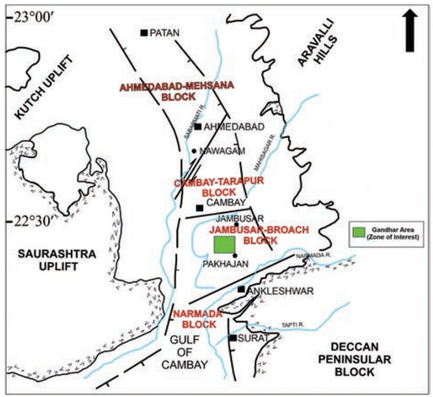Figure  1  Tectonic map of South Cambay basin (modified after S. K. Biswas, 1994). The green area represents the study area, which lies within the rift-graben system in the Cambay basin

Download: Full-Size Img

The basin is divided into five important tectonic blocks aligned along the north–south axis. Faults that run perpendicular to the rift's axis separate the blocks, including the Sanchor–Patan, Mehsana–Ahmedabad, Tarapur–Cambay, Broach–Jambusar (Saha et al., 2004), and Narmada–Tapti blocks.

The study area in Gandhar field covers a three-dimensional (3D) prestack time migrated seismic volume of 250 square kilometers. A total of 761 inlines and 1 590 crosslines occupy this location, and the bin size is 17.5 m. Over 200 well locations are available for examination, but only 10 distinct locations were selected based on the availability of gamma-ray logs (GR), density (RHOB), and sonic (DT) data (Figure 2).

Figure  2  Spatial distribution of seismic and well-log data utilized in this analysis. The red and blue dots indicate the wells under study and other wells within the region, respectively

Download: Full-Size Img

3   Methodology

3.1   Reservoir characterization

The current study presents a comprehensive analysis of systematic processes involving seismic and well-log data for reservoir characterization. This work emphasized the importance of density and sonic logs from the ten selected wells in well-log data analysis for the development of a low-frequency acoustic impedance model through the integration of seismic, well-log, and horizon data. The results will enable the creation of an absolute acoustic impedance cube through poststack seismic inversion. Horizon picking in a 3D prestack migrated volume involved the selection of seed points for various tops and automatic tracking of picks systematically in inline and crossline directions to improve precision (Figure 3). Several horizons, including Dadhar Top, Telwa Top, Ardol Top, Kanwa, Hazad, and Cambay Shale (Figure 4), were discerned and designated in this context. The primary reservoir in the study area was Hazad Member, which is characterized by deltaic sand lobes (Aswal et al., 2013) and has twelve model-based inversion (MBI) units identified in the wells (Kumar et al., 2004). Sonic and density logs were correlated with seismic reflection data for the generation of a synthetic seismogram. Then, horizons were selected using well picks to guide the subsequent process, i.e., the initial model interpolation during seismic inversion.

Figure  3  3D seismic cube featuring a specific inline where the seismic strength is consistent for efficient interpretation

Download: Full-Size Img

Figure  4  Wells intersecting with the interpolated horizons: Dadhar, Telwa, Ardol, Kanwa, and Hazad tops, along with the Hazad bottom/Cambay shale top horizon across the seismic section. The color scale represents depth values

Download: Full-Size Img

Seismic inversion was utilized to transform seismic interface properties into layer ones for the interpretation of reservoir properties. MBI was selected for its superior outcomes (Maurya and Singh, 2019), that is, the integration of various data sources for accurate findings in the acoustic impedance domain. The wavelet, which was extracted from seismic traces, was obtained using the seismic-to-well-tie method. In this study, the seismic data were in the range of 10-70 Hz and lacked low and high frequencies, which hindered the calculation of absolute acoustic impedance. Model-based poststack inversion used the seismic data and an initial impedance model as input, incorporating low-frequency information derived from well logs and constrained by horizons. The initial model incorporates low-frequency information, which was derived from well logs and horizons that served as constraints for macro layers. This initial model broadens bandwidth, which resulted in an improved vertical resolution, reduced tuning effect, and absolute acoustic impedance rather than a relative acoustic impedance. This process also enhanced simplified stratigraphic definition, which allowed for the direct correlation with well logs. The workflow for MBI involves multiple data integration steps (Figure 5).

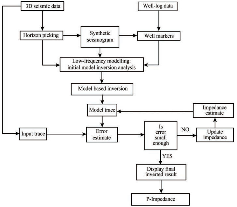Figure  5  Methodology of the applied MBI method

Download: Full-Size Img

Following inversion, porosity was predicted using impedance data, along with well-log curves and dominant frequencies from seismic data. Probabilistic neural networks (PNNs) (Maurya and Singh, 2019) were employed for this task due to their pattern recognition and classification capabilities. PNNs use Bayesian inference to estimate probability distributions, which reduces the risk of misclassification. The PNN workflow is focused on classification and pattern recognition, which is in contrast with that of the generalized regression neural network tailored for regression tasks. PNNs use independent variables to predict a single dependent variable, with the assumption of a linear combination of training data. During training, the validation errors are reduced through the determination of "sigmas" for each input attribute. A single sigma was identified, followed by the determination of an individual sigma through conjugate-gradient analysis, starting from the initial "global" sigma. This iterative process (Figure 6) improves the prediction accuracy through optimization of sigma values. Porosity served as the primary variable in the study. The neural network architecture is described as follows:

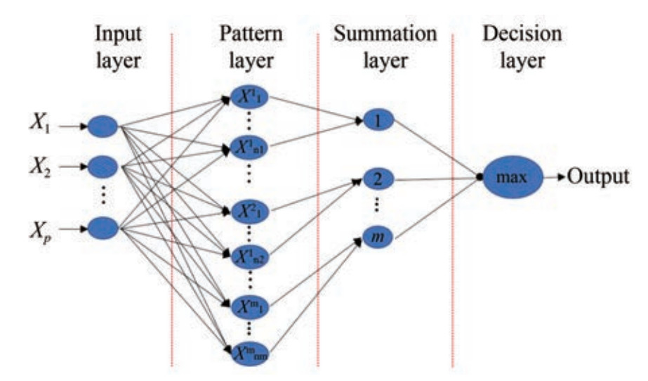Figure  6  Input, pattern, summation, and decision layers covering the entire operation of the PNN algorithm

Download: Full-Size Img

Input Layer: Each predictor variable is represented by a neuron, and N-1 neurons are employed for categorical variables. Data standardization was performed by subtracting the median from each data point and then dividing the result by the interquartile range. This process normalizes the data, reduces the impact of outliers, and ensures uniform data scales.

Pattern Layer: Neurons store predictor variables and target values. A hidden neuron is used to calculate the distance between a test case and its center point. Then, a radial basis function is applied using sigma values.

Summation Layer: Each target variable category exhibits a pattern neuron. Hidden neurons store the actual target category, and their weighted outputs are inputted to the corresponding pattern neurons whose values are aggregated.

Output Layer: This layer compares the accumulated weighted votes from pattern neurons for prediction of the target category.

Further assessment of the geophysical interpretation is elucidated in the subsequent Results section. This part of the paper delineates the methodology for wavelet selection to achieve optimal synthetic seismograms at well locations, construction of the P-impedance model, correlation of the original and inverted logs, and selection of seismic attributes for the generation of a desired porosity volume employing PNN.

3.2   Geomechanical modeling

3.2.1   Overburden stress

The overburden pressure S_v (z) at any depth refers to the pressure resulting from the combined weights of the rock matrix and fluids in the pore space overlying the formation of interest (Zoback et al., 2003). This relation is expressed as follows:

where ρ_b indicates the depth-dependent bulk density given by the following.

where ϕ, ρ_f, and ρ_g denote the fractional porosity, pore fluid density, and density of the matrix (grain density), respectively.

The effective stress S' refers to the stress acting on the solid rock framework. According to Terzaghi's principle, effective stress is defined as the difference between the overburden pressure S_v and the pore pressure P_p (Terzaghi, 1943):

The effective stress S' controls the compaction process of sedimentary rocks; any condition at depth that causes a reduction in S' will also reduce the compaction rate and cause overpressure.

3.2.2   Pore pressure estimation

Eaton's sonic method is often applied in the estimation of pore pressure in subsurface formations. The procedure is based on the relationship between compressional wave velocity and pore pressure. The principle behind this method is that with the increase in pore pressure, the compressional wave velocity decreases due to the reduced effective stress on the rock matrix caused by the increased fluid pressure. Therefore, the compressional wave velocity can be used to estimate pore pressure (Eaton, 1975):

where P_p refers to pore pressure, V_p denotes the compressional wave velocity, V_s indicates the shear wave velocity, ρ_w represents the density of water, ρ_m stands for the density of the rock matrix, φ is porosity, Δt corresponds to the time difference between compressional and shear waves, and t means the travel time for compressional wave.

Eaton's sonic method requires the measurements of compressional wave velocity and porosity. The compressional wave velocity was measured using a sonic logging tool, which sends high-frequency sound waves through the formation and measures the time required by waves to travel from the source to the receiver. Porosity can be determined from Nuclear Magnetic Resonance (NMR) logs or core samples (Freedman et al., 1997; Tariq et al., 2022).

It is important to note that Eaton's sonic method has limitations and is subject to various assumptions and uncertainties, such as the assumption of constant porosity and density throughout the formation. Therefore, it is often used in conjunction with other methods for pore pressure estimation and validated using additional data, such as mud weight and drilling parameters.

3.2.3   Fracture gradient

Fracture gradient describes the amount of pressure required to cause fracture in rock formations. It is usually expressed in pounds per square inch (psi) or kilograms per square centimeter (kg/cm²). The estimation of fracture gradient in drilling operations ensures that the pressure exerted by the drilling fluid does not cause damage to formation integrity. If the pressure exceeds the fracture gradient, the drilling fluid can penetrate the formation and considerably damage the well, which will incur high repair costs. Similarly, if the pressure buildup from subsurface CO₂ injection exceeds the fracture gradient, it can damage the reservoir and caprock. This condition can also trigger the reactivation of dormant faults and the creation of new fractures that can act as leakage pathways for CO₂ to the surface. The fracture gradient can vary depending on the type of rock formation and well location, and thus, it must be determined prior to CO₂ injection.

4   Results

4.1   Reservoir characterization

A close match between the synthetic seismogram and seismic reflection data was required. The well-to-seismic tie process involved the statistical extraction of a wavelet from seismic data (Shao-wu et al., 2009; Wang et al., 2017), with horizons serving as reference points, correlation of logs with seismic data, attainment of a wavelet, and repetition of the process for all available wells. Single-wavelet seismic inversion is obtained by averaging and correlating wavelets at each well until an acceptable correlation has been reached (Figure 7(a)). Figure 7 shows the seismic-to-well tie process demonstrated using a statistical wavelet of length 200 ms and the 89% correlation observed in the reservoir zone. The synthetic seismogram (blue) displayed in Figure 7(a) matched the seismic traces shown in red and thus provided a distinct comparison between synthetic and actual data. After the seismic-to-well tie process, a synthetic seismogram was generated, and a synthetic trace was overlaid on the seismic data for well GND-002 (Figure 8).

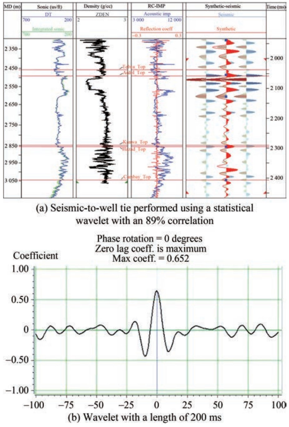Figure  7  The traces in blue and red (a) represent the synthetic seismogram and actual seismic trace on the second track from the left

Download: Full-Size Img

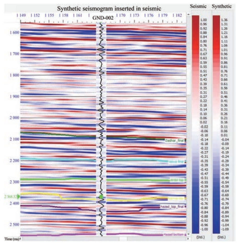Figure  8  Results of the seismic-to-well tie process. The added synthetic (black) curve overlaid the seismic data for well GND-002. The visible horizons include the Dadar, Telwa, and Hazad tops and Hazad bottom/Cambay shale tops

Download: Full-Size Img

4.2   Impedance model

The seismic and synthetic seismic data exhibited a satisfactory correlation, which prompted the development of an initially low-frequency P-impedance model (Figure 9). The model underwent multiple iterations until the final inverted model was achieved to minimize the error between synthetic seismic traces and the observed seismic data. The least-square technique was used to execute the inversion process.

Figure  9  The inserted curve represents P-impedance. The color scale illustrates the P-impedance values of the initial model, specifically the low-frequency model, where the red and green colors indicate high and low P-impedance values, respectively

Download: Full-Size Img

Figure 10 displays the more than 90% correlation observed between synthetic seismic and original seismic data in most well locations, which indicates a high level of accuracy. This high correlation allowed for confidence in proceeding to the final inversion step.

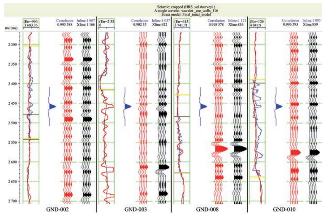Figure  10  Poststack seismic data on the leftmost log results, with the red and blue curves indicating the inverted P-impedance and original impedance result, respectively. The correlation between the synthetic trace (red) of the blind wells GND-008, 010, and seismic trace (black) exceeded 90%. The blue curve depicts the wavelet employed in convolution to generate synthetic seismic traces. The analysis covered four wells, and the wavelet used for each well was the average wavelet generated earlier

Download: Full-Size Img

After the creation of the initially low-frequency model and a quality control assessment for the evaluation of the efficacy of inversion results, the final inversion step was set for implementation. In this stage, the final inversion process determined an inverted acoustic impedance log at each well location. This process entailed the interpolation between wells to generate a comprehensive inverted cube with acoustic impedance. Quality control was performed to identify the effectiveness of inversion. Thus, a cross plot (Figure 11) was used to compare the predicted and actual acoustic impedances. The correlation error along each well was checked, and based on the error margin, the wells were selected for inversion at a later stage. However, the number of iterations is a critical parameter, and high errors may emerge if they exceed a specific limit. Figure 11 depicts a one-to-one comparison of the inverted sample and actual acoustic impedance at the blind well locations GND-008-010, which revealed a commendable correlation of 87%. This correlation represents the accuracy and reliability of the final inversion results.

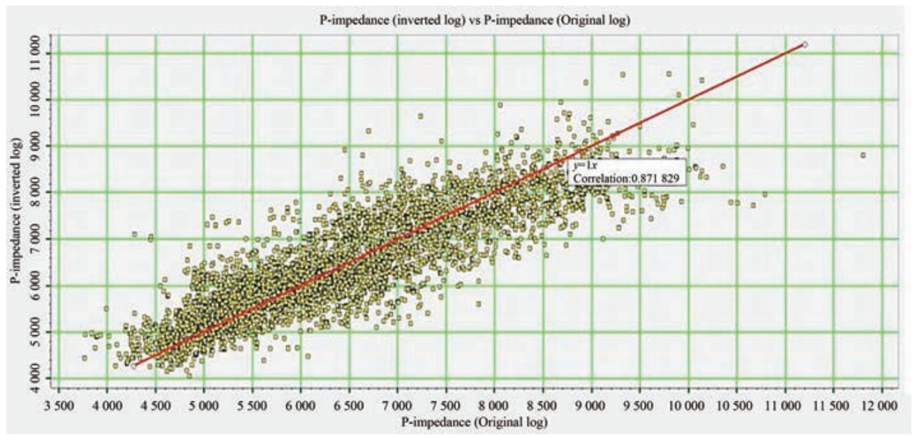Figure  11  Correlation between the P-impedance of the original logs and all inverted logs. A robust correlation of 87% was achieved for the blind wells GND-008, 009, and 010, which indicates a favorable condition to proceed with further inversion analysis

Download: Full-Size Img

4.3   Porosity estimation

To estimate the log property volume for all locations in the seismic volume, we utilized the relationship between seismic data and well logs. Our goal was the identification of an operator that can accurately predict well logs based on attributes of nearby seismic data, potentially through nonlinear means. This approach allows for the creation of new well logs, which can then be used for cross-sections, attribute volumes, and mapping purposes. The study aimed to discover density porosity as the target property.

Various methodologies exist to address the challenges in porosity prediction. Among them, neural networks are identified as one of the most effective algorithms (Maurya and Singh, 2015). In this research project, we extended our approach by conducting single- and multiple-attribute analyses and employing PNN techniques.

4.3.1   Single-attribute analysis

Single-attribute analysis is a linear regression method that evaluates all possible combinations of seismic attributes to predict the porosity of the target zone. However, the large number of attribute combinations often causes inaccurate predictions as numerous attributes may be unrelated to the porosity. Table 1 demonstrates the model correlation with porosity calculated separately for all attributes. For the prediction of porosity, a linear regression technique was used to explore all possible combinations of seismic attributes. However, not all attributes establish a meaningful relationship with porosity. As a result, less accurate predictions may be obtained due to the vast number of attributes and combinations.

4.3.2   Multi-attribute analysis

This study explored methods for the analysis of multiple attributes to predict a single variable, porosity, by testing attributes to determine the combination of attributes that best predicts the target. Two common approaches are used for searching multiple attributes. The first approach is an exhaustive search involving tests for all possible combinations and selecting those with the least prediction errors. However, this method is computationally intensive and requires significant resources. The second approach is step-wise regression, which identifies the best single attribute (Table 1), followed by the best pair of attributes, and so on. At each step, the root mean square prediction error was used to select the optimal attribute combination. The latter method was selected as our preferred approach. Figure 12 displays the training window for multiple-attribute analysis, displaying the modeled (red curve) and actual (black curve) density porosity log curves for multiple wells. The analysis window was delineated by a horizontal yellow line, within which various analyses were conducted for the comparison of the modeled and observed density porosity values across wells. The results show that the modeled density logs fall within the range of the original density logs and exhibit a close match to them.

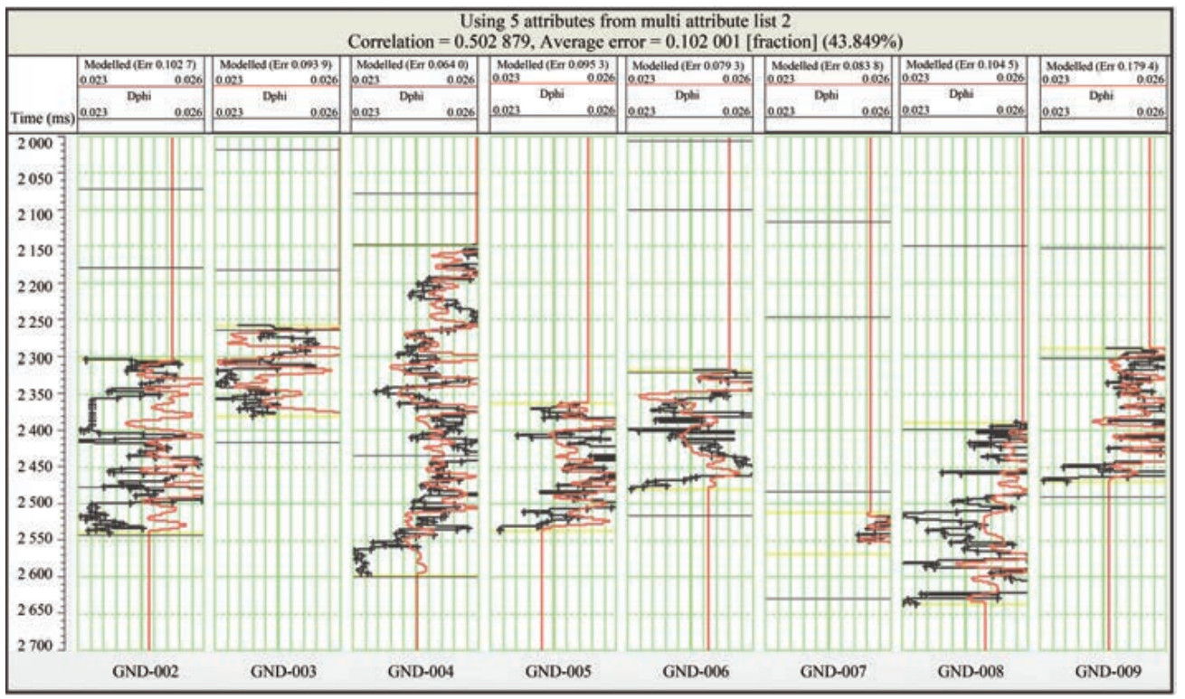Figure  12  Training window for multiple-attribute analysis. The red and black curves show the modeled and actual density porosity, respectively, for multiple wells. The analysis window is within the yellow horizontal lines

Download: Full-Size Img

4.3.3   PNN training

PNNs possess a structure similar to that of a feedforward neural network, with input, pattern, summation, and output layers. The main objective was to obtain the highest correlation and minimal validation error through PNN analysis. Figure 13 presents the error in PNN analysis for the studied wells.

Figure  13  Error graph for the PNN analysis at various wells

Download: Full-Size Img

PNNs are widely used in classification tasks, and they show high effectiveness in establishing nonlinear relationships between seismic and well data. Accurate results in porosity prediction were obtained using a multilayered PNN with input, pattern, summation, and output layers. Figure 14 shows the 98% correlation between the predicted and actual porosities during the training.

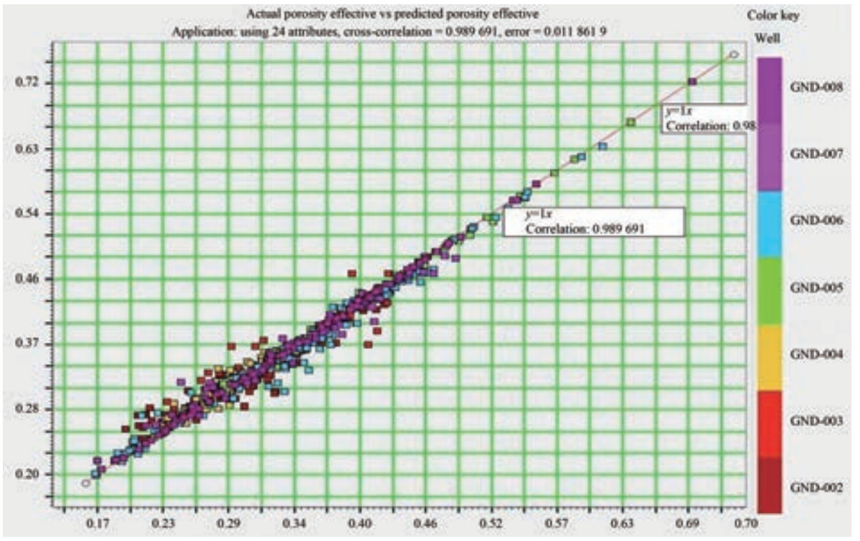Figure  14  Predicted and actual porosities during training showed a 98% correlation between data. The legend shows the colors used for various wells

Download: Full-Size Img

4.3.4   PNN validation

Validation was performed on the wells logs that were left blank during training. Figure 15 shows the black and red traces, which represents the actual effective and estimated porosity values, respectively. The error in the model is below 5% in the two test wells (GND-001 and GND-009). The test set provides a distinct indication of the various attributes that have been trained on the training data and are functioning in positions distant from the training well.

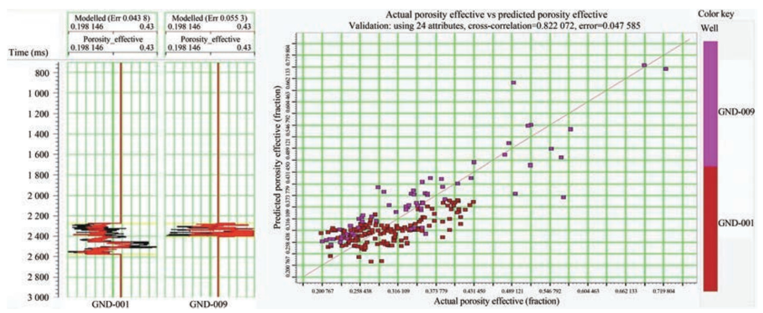Figure  15  (a) Blind validation test on the wells during training. The black and red traces represent the actual effective and predicted porosities, respectively; (b) Correlation (82%) between the actual and predicted effective porosities after validation. The red dots represent the wells GND-001, and the purple line denotes well no GND-002

Download: Full-Size Img

4.3.5   Porosity volume estimation

Total porosity is calculated using density porosity and neutron porosity. We were provided with neutron porosity using the well-log data, and density porosity was calculated using the density log. From these, total porosity is determined, which is our target property. The same steps used in the calculation of density porosity are repeated for the estimation of total porosity. We employed impedance, derivative, instantaneous phase, integrated, and quadrature trace attributes for multiple attribute analysis.

The effective porosity distribution in the volume is displayed, with well GND-003 (Figure 16) considered a reference point. The porosity values from the well aligned remarkably with those obtained from the PNN. The target zone was between the Hazad top and Hazad bottom, with porosity variation observed between them. This decrease was reflected in the impedance data, with the same horizon exhibiting an increased impedance compared with the surrounding areas.

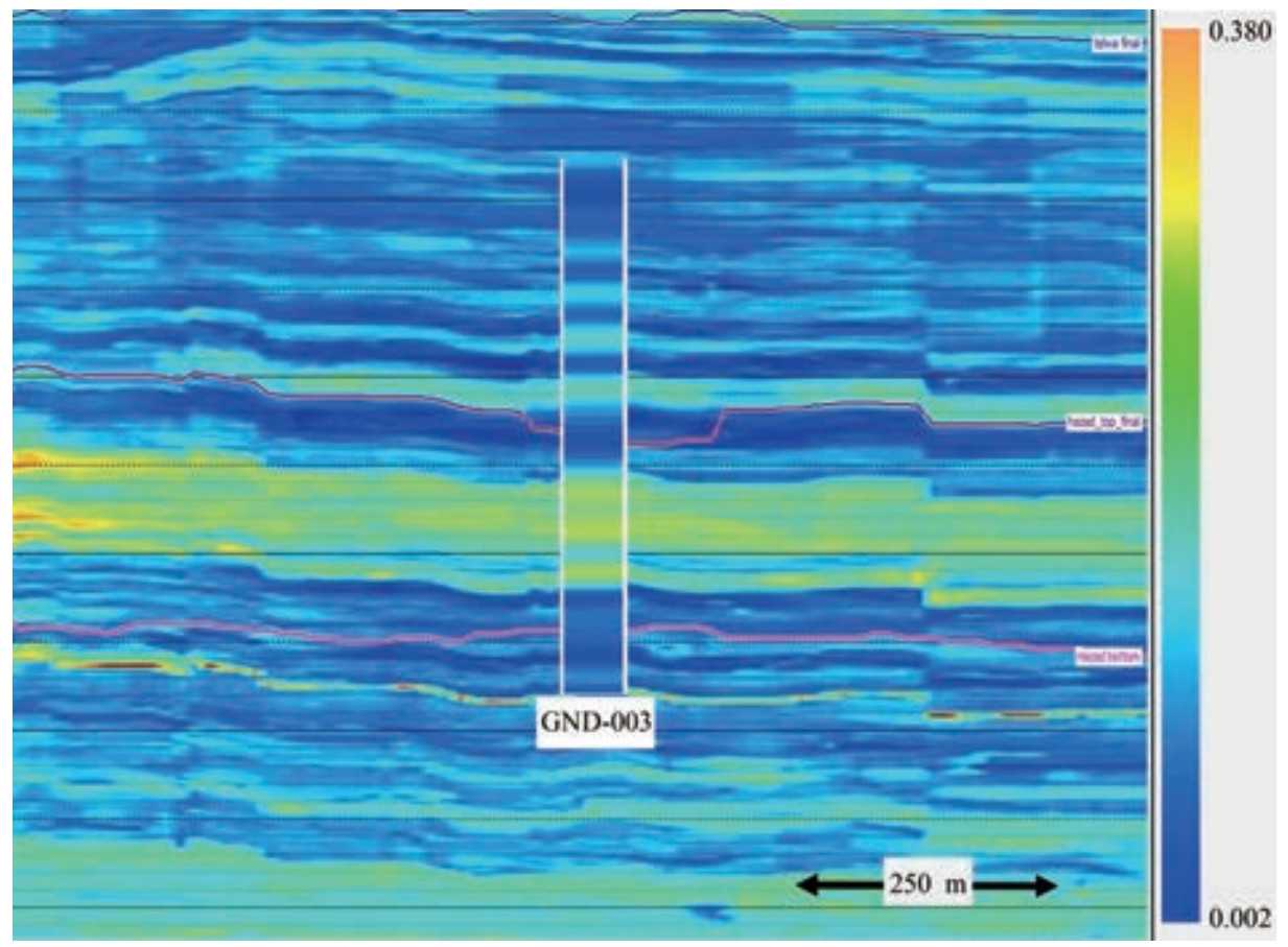Figure  16  Effective porosity observed at well GND-003, wherein a congruent correlation was evident between the porosities derived from well data and seismic analysis

Download: Full-Size Img

4.4   Geomechanical model

Following a meticulous analysis of over 60 well bores in the studied region, we identified two vertical wells, namely, GND-011 and GND-012, as optimal selections for the establishment of a reliable geomechanical model under in-situ pressure conditions. These wells exhibited the most extensive coverage in petrophysical logs and provided well-calibrated information, which made them suitable for the development of a robust geomechanical model. Table 2 encompasses the comprehensive inventory available in the studied wells. Figure 17 presents a well-log composite view and illustrates the available log curves essential for our study.

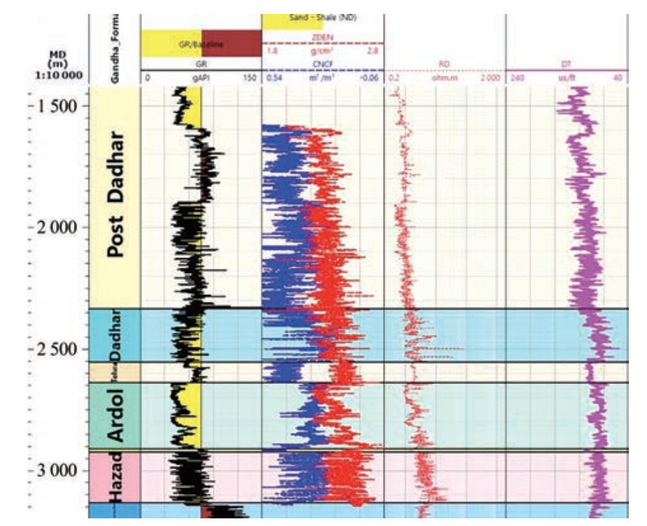Figure  17  Availability of well logs in GND-012 borehole

Download: Full-Size Img

We used the available well-log data to calculate the overburden stress, pore pressure, and fracture gradient. The obtained results were used to evaluate of the geomechanical feasibility of CO₂ sequestration in the reservoir.

4.4.1   Overburden stress analysis

Calculation of overburden stress necessitated the acquisition of density data from the well's inception. However, starting at 1 580 m, the initial density log data showed a data gap. To overcome this limitation, we generated a synthetic density profile based on the density values of neighboring geological layers. This synthetic profile attained a seamless integration with the actual well-log density data, which filled the depth range initially devoid of data. This approach ensured the completion of the density dataset required for precise overburden stress calculations, which facilitates the comprehensive analysis of subsurface conditions. The vertical stress (Sv) and overburden gradient (OBG) profiles for well GND-012 were determined using density log data. Missing data in the shallow region were addressed using an extrapolation method, with the exponential curve from the surface to the first density data point. The fitting equation for this extrapolation curve is y = c + ae^xb. This mathematical model was used to estimate the density values in the shallow portion through extrapolation from available data points. Subsequently, the data were utilized to calculate Sv and OBG profiles (Figure 18). The prior estimation of necessary input parameters in the earlier step enabled a straightforward estimation of overburden stress.

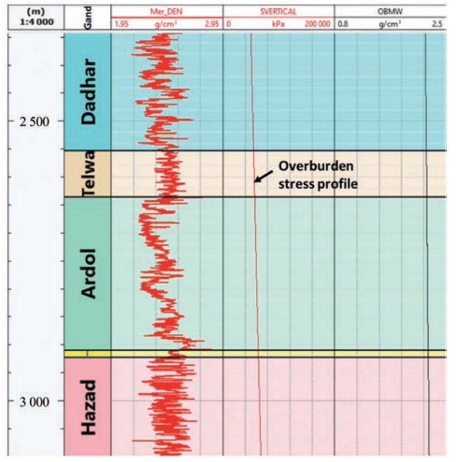Figure  18  Overburden stress gradient profile derived from density log data

Download: Full-Size Img

Calculation of overburden stress was followed by estimation of the pore pressure profile along the stratigraphic succession. The pore pressure initially followed a hydrostatic trend until the bottom section of the Telwa Formation was reached. Subsequently, the Hazad Member revealed a gradual increase in the pressure gradient to approximately 9.4–9.5 pounds per gallon (ppg).

4.4.2   Pore pressure

Eaton's sonic method was used to estimate the pore pressure. The input logs utilized for this computation comprised gamma ray, compressional slowness, and density. The plots reveal the mud weight equivalent and absolute pressure alongside the overburden stress and hydrostatic pore pressure (Figure 19) and an overpressure zone within the formation was identified.

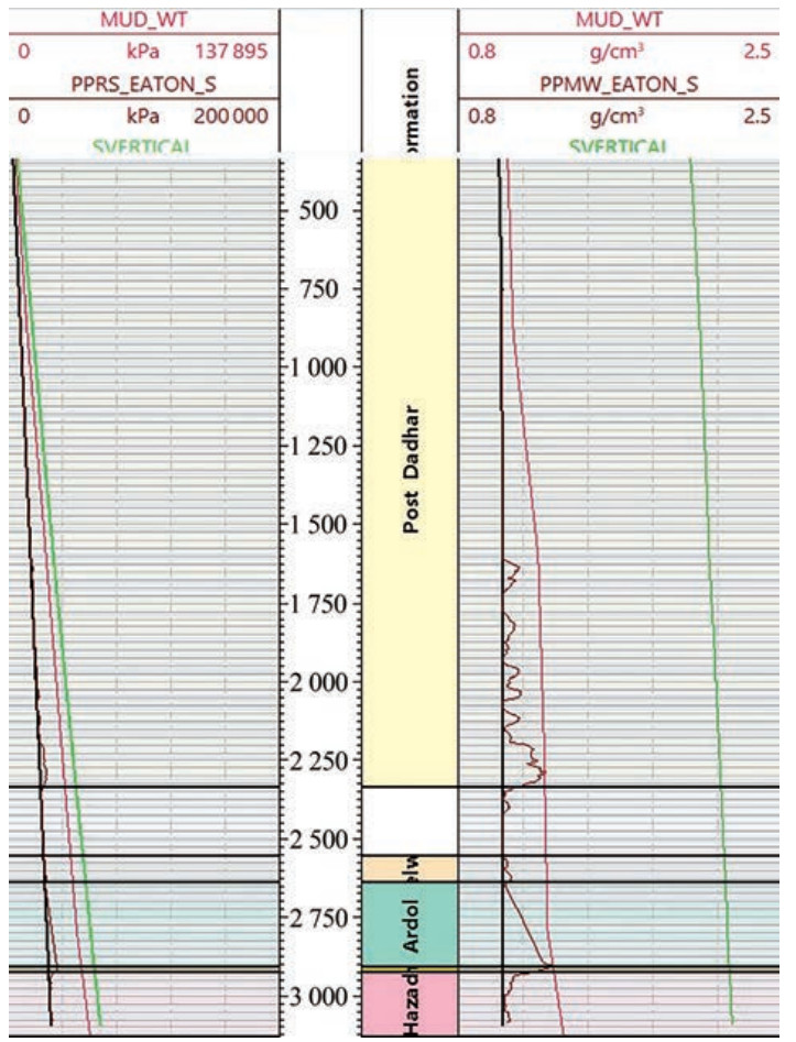Figure  19  Pore pressure profile estimated from log data

Download: Full-Size Img

The findings suggest that certain areas within the formation experience subsurface pressures that exceed the expected values based on the overburden stress alone. Comprehension and identification of such overpressure zones are critical for drilling and reservoir management, as they can affect drilling safety and wellbore stability.

For the mud weight calibration process, a plot incorporating mud weight and pore pressure plots was created (Figure 19). The pore pressure curve calculated using Eaton's sonic method demonstrated reasonable accuracy during the calibration with mud weight and drilling events. Thus, this method was preferred for the calculation of fracture gradient and other subsequent calculations.

4.4.3   Fracture gradient

The fracture gradient is a vital parameter in CO₂ storage operations, where the increased pore pressure from CO₂ injection can result in rock failure. Such a condition can cause damage to the reservoir and caprock and ultimately influence the containment of CO₂ in the subsurface. Estimation of fracture gradient then becomes essential to comprehending the maximum pore pressure buildup that the formation can accommodate and, consequentially, the pressure-constrained storage capacity of the reservoir. The rock mechanical parameter ultimately aids in planning CO₂ injection operations, such as injection rates and target locations, which considers various factors, such as the mechanical properties of rock formation, overburden stress, and pore pressure. The fracture gradient plot spanning Dadhar to Hazad intervals displayed the pore pressure calculated using Eaton's formula along with mud weight (Figure 20). The mud weight and pore pressure were considerably below the fracture gradient, which indicates a negligible risk of fracture formation. This finding also indicates that the reservoir can accommodate further pore pressure buildup and provides confidence for future CO₂ injection.

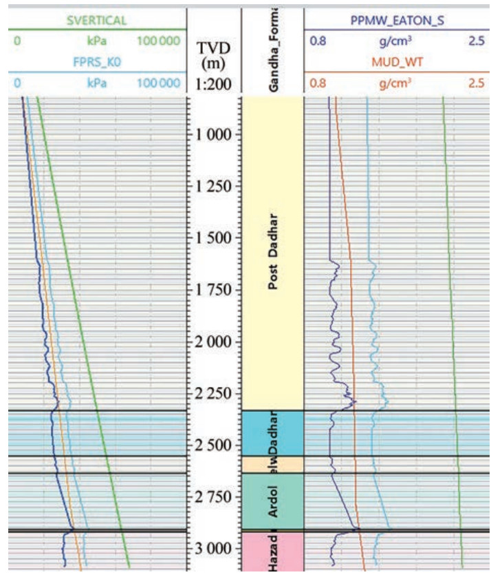Figure  20  Fracture gradient in relation to pore pressure, mud weight, and Sv in the well

Download: Full-Size Img

5   Discussion

The seismic inversion process covered the entire seismic volume with specific parameters and involved iterative adjustments to minimize differences between seismic and synthetic seismic traces. To maintain fidelity, we implemented constraints on impedance changes while referencing the model's average impedance from the filtered well impedances. The inversion results at the well were compared with the well-log data impedance using a high-cut filter to the well-log data to accommodate its higher frequency relative to seismic data.

The MBI algorithm used in this work divides the zone into layers or blocks to generate pseudovelocity logs. The final model was synthesized using the blocked model and the wavelet, which resulted in a synthetic trace that aligned with the actual seismic trace. Alignment was improved through iterative adjustments to layer thickness and amplitude, with a constant number of blocks maintaining a consistent average block size. A coarse structure was obtained with the application of large intervals, whereas smaller intervals improved resolution at the expense of runtime.

The inverted acoustic impedance exhibited a superior resolution compared with the observed seismic data. Figure 21 illustrates the robust 87% correlation noted between the P-impedance of the original and all inverted logs, which provided substantial support for further analysis. The 3D P-impedance cube visually represented the acoustic impedance around the wells, which delineated horizons, such as Dadhar, Telwa, and Hazad tops and Hazad bottom in Figure 22. This comprehensive representation underscores the effectiveness of seismic inversion methodology in the characterization of seismic facies (Xu and Haq, 2022) and improved comprehension of geological features.

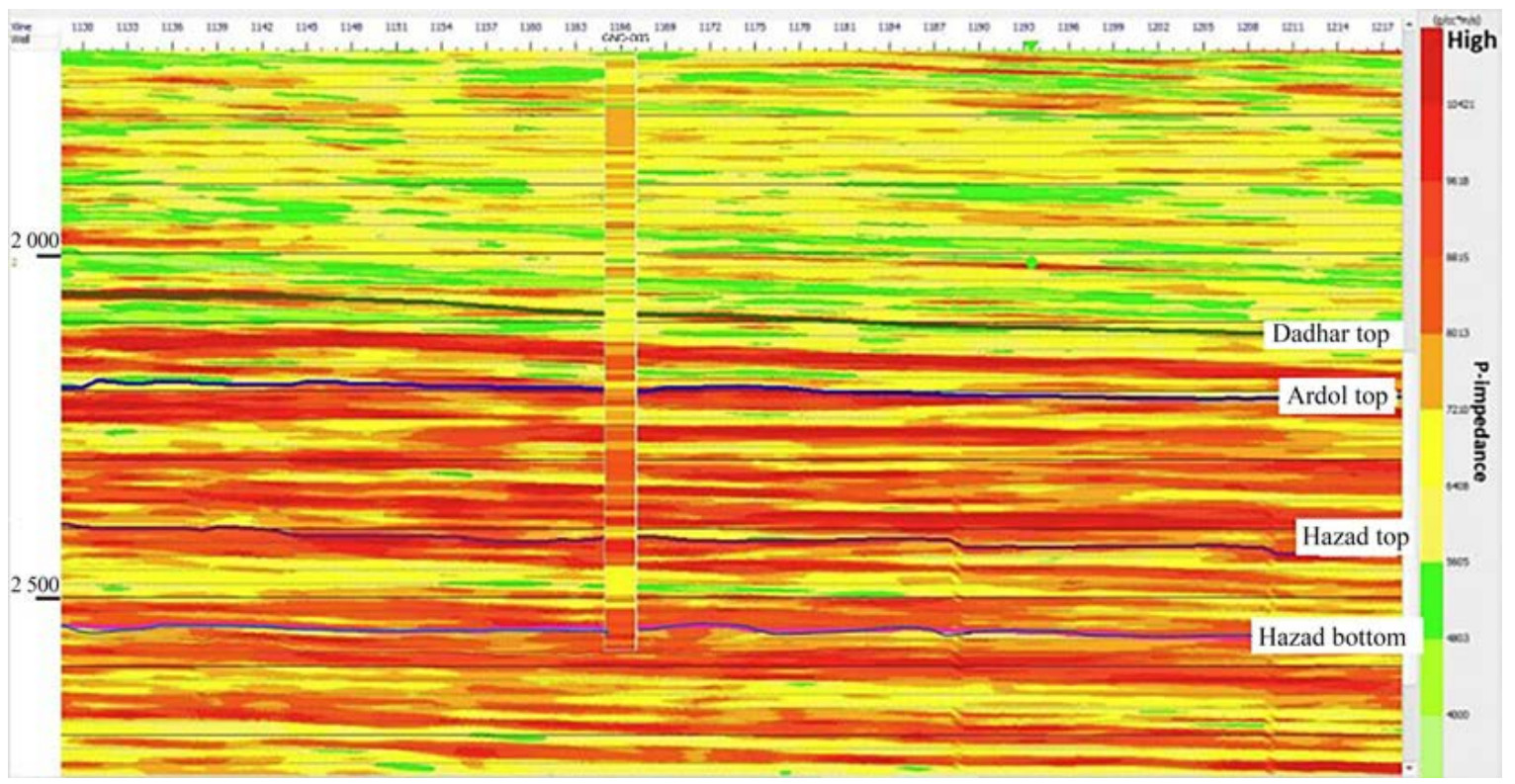Figure  21  Model-based poststack seismic inversion results around the well GND-005 in the inline section. Blue curves mark the horizons, and the color bar signifies acoustic impedance values, where red and green colors indicate high and low acoustic impedances, respectively

Download: Full-Size Img

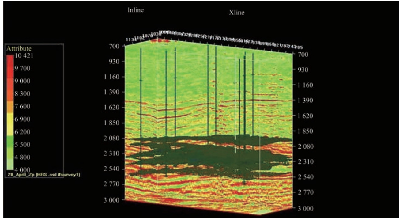Figure  22  3D P-impedance cube providing a view of the acoustic impedance distribution around the wells, accompanied by the display of horizons, such as Dadhar, Telwa, and Hazad tops and Hazad bottom (arranged from top to bottom)

Download: Full-Size Img

However, the correlation between inverted and actual acoustic impedance curves at well locations can be increased using parameters such as wavelet frequencies or different wavelets. This information was reverted to the seismic-to-well-tie process to obtain a better correlation.

The analysis of literature particularly centered on the Hazad Member, highlights clastic sedimentation occurring within a marine environment (Jaiswal et al., 2018). Alongside the observed onlapping and downlapping terminations, the sediments displayed a noticeable parallel arrangement (Figure 21). The fragmented sands (in red), which were characterized by high impedance, were supported by conventional core data, which indicates their deltaic nature. Conversely, in other areas, the sands contained more shale content, which is abundant throughout the Hazad section. Thus, the formation represents a shale-rich system, indicative of a period of transgressive sediment deposition.

For determining the porosity of geological formations, the interplay between velocity and density must be considered as these produce acoustic impedance. Accurate porosity calculations were ensured via multi-attribute analysis, which included a broad range of attributes, such as impedance and density, that led to improved results. This finding highlights the interconnected nature of porosity and the geological attributes. To anticipate porosity and to ascertain reservoir characterization, we explored neural network models and identified PNN as the most efficacious, primarily due to its sophisticated internal network (Maurya and Singh, 2015; Maurya et al., 2020). The PNN model underwent twenty-five (25) iterations, which was determined to be the optimal number to prevent overtraining.

In this study, reservoir modeling contributed to the exploration of the heterogeneity of thin sand within the transgressive sediment pack. The simulations conducted in this research were used effectively in the examination of geological carbon sequestration in subsurface rock formations. This work is unique in its field and the first of its kind. Seismic analyses provided a regional-scale understanding, complemented by well data. However, the lack of core information may influence calibration during prediction. Nevertheless, the close match between porosity data from wells and porosity volume instills confidence in reservoir simulation. However, porosity alone does not determine the volumetric capacity of reservoirs. Reservoirs also possess a dynamic pressure-limited capacity that increases gradually over time with injection. Specifically, pressure buildup during the initial injection phase limits reservoir storage capacity in the short term, while volumetric capacity becomes the primary constraint in the long term (Szulczewski et al., 2014). Therefore, insights into the limitations in storage capacity due to pore pressure buildup from CO₂ injection must be obtained (Bachu, 2015, 2016). Analysis of reservoir pore pressure profiles and estimated fracture gradients for the the Gandhar field indicate ample room for further pressure buildup. This analysis provided valuable insights into reservoir and wellbore stability, which can aid in the mitigation of potential geomechanical issues, including induced seismicity. However, site-specific storage planning necessitates further analysis and risk assessment before injection.

6   Conclusions

Site screening studies are imperative for the development of CO₂ storage in India. In this work, we characterized the CO₂ storage potential of the Hazad Member in the Gandhar field in the Cambay basin. Seismic data were integrated with well-log data. Machine learning was used to predict variations in the total porosity across the target zone based on the relationship between acoustic impedance and total porosity at individual well locations. Our results revealed that effective porosity exceeded 25% in several areas within the Hazad Member, suggesting well-connected pore spaces conducive to efficient CO₂ migration. Based on our literature survey, we proposed the categorization of reservoirs into different ranks depending on their propensity for CO₂ storage. As a result, we managed to identify the most prospective regions within the zone of interest and observed the overall performance of the reservoir to be conducive to storage. Corroborating the distribution of porosity with the GR log through cross-plots enabled the prediction of the lateral continuity of sand lithofacies. We also performed geomechanical studies to gain insights into various constraints in storage capacity, address risks related to leakage, seal integrity, and induced seismicity, and evaluate the limits for safe CO₂ storage. The vertical stress in the Hazad Formation ranged from 63 MPa to 68 MPa, and the pore pressure from 30 MPa to 34 MPa due to depletion staying significantly below the fracture gradient, indicating minimal risk of fracture during CO₂ injection. The analysis confirmed that the Hazad Member in Gandhar field possesses substantial potential for CO₂ storage with sufficient porosity and geomechanical stability, making it a promising site for carbon storage. Having identified potential sites for CO₂ injection, we propose flow modeling studies at the reservoir scale for comparison of the migration pathway of CO₂ under various injection scenarios as the next step.