1   Introduction

With the development of shipping trade, the port container throughput has been rising continuously. In fact, China's container throughput had grown from 163.67 million TEU in 2011 to 296 million TEU in 2022 according to data from the Ministry of Transport. As the load of container terminals continues to increase, this leads to greater requirements for the efficiency of terminal operations. At the same time, this promotes the reform and innovation of container terminal facilities and equipment, along with loading and unloading processes. Among them, "quay crane(QC) + AGV + automatic rail-mounted gantries (ARMG)" and "quay crane + container truck + ARMG" are the two most typical loading and unloading processes in current automated container terminals. As such, many scholars have studied the problem of collaborative scheduling of equipment resources within these two loading and unloading processes.

For example, regarding the joint scheduling study of automated container terminals, Meersmans and Wagelmans (2001) first proposed the joint loading and unloading operation process of AGV, quay crane, and ARMG in the automated terminal. Then, they used the directional search and branch and bound methods to obtain the minimum completion time. Kim and Lee (2010) proposed a schedule improvement algorithm based on a simple neighborhood search. They referred to the results of Meersmans and Wagelmans (2001) to study all operations of automated stacking cranes (ASCs), rail-mounted gantry cranes, and automated guided vehicles (AGVs) with the goal of improving the efficiency of automated container terminals. The method is also evaluated using a simulation study. Dkhil et al. (2013) similarly optimized the QC-AGV-ASC planning problem in automated container terminals by proposing three mathematical models with the aim of minimizing the loading time and the number of vehicles required. The first model considers a single QC and a single ASC, the second model considers multiple QCs and a single ASC, and the third model considers multiple QCs and multiple ASCs. In addition, the solution was performed using Cplex. Skinner et al. (2013) studied the scheduling of several types of equipment in a container terminal. A genetic algorithm (GA)-based optimization method is proposed to reduce the overall time cost of container transportation at automated container terminals. Homayouni et al. (2012) considered a split-platform automatic storage/retrieval system for the integrated scheduling problem of loading and unloading equipment in automated container terminals. Then, they developed a mixed-integer programming model, along with a simulated annealing algorithm, to find a near-optimal solution to the problem in a short time.

Yang et al. (2018) investigated the integrated scheduling of QC, AGVs, and ARMGs, along with the path planning problem of AGVs, to reduce the conflict and congestion problems of AGVs as a way to improve operational efficiency. In their paper, a two-level programming model is proposed, and a congestion prevention two-level GA (CPR-BGA) is designed to solve the model. Zheng et al. (2010) proposed an integrated equipment scheduling model for an automated container terminal using twin 40' cranes. The proposed model generates equipment scheduling plans as well as yard storage plans and vessel allocation plans guided by the goal of reducing the turnaround time of each container vessel that stays at the berth. An efficient heuristic is also designed to solve the integrated scheduling problem. Numerical experiments show efficient performance and satisfactory results. Tang et al. (2014), Wu (2018), and Kaveshgar et al. (2015) developed mixed-integer programming models for the joint scheduling of quay cranes and container trucks as well as designed improved PSA, GA and GA combined with a greedy algorithm to solve the problem of loading and unloading operations. Cao et al. (2010a, 2010b) proposed a mixed-integer programming model for the coordinated scheduling of a single quay crane and multiple container trucks. They also proposed an integrated scheduling model for container trucks and ARMGs. The former used GAs and improved Johnson's rule heuristics algorithm to improve the efficiency of the solution, while the latter solved the problem of the Benders mutation.

Han and Mou (2014) established a cooperative scheduling model for quay cranes and container trucks considering the uncertainty of container truck arrival time. Their objective was to minimize the completion time of container trucks and solve the problem using an improved GA. Meanwhile, Lu and Le (2014) developed a model to minimize the total working time of the quay crane, the container truck, and the ARMG, considering several factors, including the uncertainty in the travel speed of the internal container truck, the horizontal running speed of the ARMG and the loading and unloading speed. They were able to solve this using a particle swarm algorithm (PSA). Lau and Zhao (2008) proposed a mixed-integer programming model for the integrated scheduling of QC, AGVs, and automated yard cranes (AYCs). Their proposed model refines the inter-equipment constraints and considers the loading and unloading bidirectional flow problem with the aim of minimizing the operational delays of QCs and the total travel time of AGVs and AYCs. They also proposed a heuristic called multilayer GA (MLGA) for obtaining near-optimal solutions to the integrated scheduling problem and an improved heuristic called GA plus maximum matching (GAPM) to reduce the computational complexity of the MLGA method. The performance of GAPM is also compared with that of the MLGA method. Tian et al. (2018) took time minimization as the goal and considered the mode of loading and unloading operations to establish a mixed-integer programming model. They then adopted the multilayer GA and the cooperative scheduling method, combining GA and heuristic strategy to solve the problem.

Heuristic algorithms, such as PSA and simulated annealing (SA) algorithm, have been widely used in solving the cooperative scheduling optimization problem of automated container terminal equipment. For example, Liu and Liu (2016) proposed a cooperative scheduling model for quay cranes and container trucks. The proposed PSO-AFSA, which combines the global optimal search capability of the particle swarm optimization (PSO) algorithm and the powerful local search capability of the artificial fish swarm algorithm (AFSA), aims to solve the problem by generating multiple primitive paths for selecting the set of nodes for the optimization problem, thus avoiding the prematureness of PSO. Hsu and Wang (2020) studied the berth allocation and shore bridge scheduling problem and attempted to use various heuristic/metaheuristic methods, including first-come, first-served (FCFS), PSO, modified PSO (PSO2), and multi-PSO (mPSO), to determine a better approach. Subsequently, Hsu et al. (2021) investigated the scheduling export container problem using both yard cranes and yard trucks in the container terminal yard side area. They assembled load balancing heuristics, GA, and PSO to develop an ensemble SGPSO algorithm for solving the problem. Simulation results indicated that the SGPSO outperformed the single algorithm. Jonker et al. (2021) used a hybrid flow shop format to construct a bidirectional flow operation scheduling model for automated container terminals. The coordination model is solved by a tailored SA algorithm. Nourmohammadzadeh and Voss (2022) proposed an integrated multiobjective mathematical model that considers the uncertainty of the arrival time of vessels and the failure time of quay cranes, which may vary depending on certain scenarios. The exact solutions to small-scale problems were obtained using Gurobi software. Meanwhile, for large-scale complex problems, two SA-based meta-heuristics were used for the solution: multiobjective SA (MOSA) and Pareto-simulated annealing methods with a new solution encoding scheme. The PA has the advantages of fast convergence and simple structure, but its search accuracy is low, and it tends to fall into local convergence during the solution process. In comparison, the SA algorithm can accept solutions worse than the current one with a certain probability. In this way, it is possible to exceed the local optimal solution and reach the global optimal solution.

Some scholars have successfully combined the two algorithms and applied them to the solution of various optimization problems. For example, Abbaszadeh et al. (2021) developed a mixed-integer linear programming model to minimize the maximum completion time in flexible flow shop scheduling problems. They then proposed two metaheuristic algorithms (PSO and hybrid SA-PSO) to solve the model. The numerical experiments show excellent results. Furthermore, Abbaszadeh et al. (2021) reported that the SA-PSO algorithm can be extended to other scheduling problems involving renewable resources and multiple objectives. Other scholars have applied the SA-PSO algorithm to parameter optimization problems. For example, Liu et al.(2022) introduced the SA algorithm into the traditional PSO algorithm to form an adaptive SA-PSO algorithm. This algorithm enters the SA algorithm as an input quantity to calculate the probability of the particle becoming the global optimal solution and the optimal missile formation parameters after the PSO determines the individual best position and the global optimal position of a particle. Although the SA-PSO algorithm has been applied to various optimization problems, the use of such a solution to address the automated container terminal scheduling problem has not yet been realized.

Thus far, research on the collaborative scheduling of automated container terminals mostly focused on the collaborative scheduling between equipment under the two loading and unloading processes of "quay crane + AGV + ARMG" and "quay crane + container truck + ARMG." In comparison, less consideration has been given to the uncertain factors in the loading and unloading process. In actual automated terminal operations, it is becoming increasingly difficult for a single loading and unloading process to meet the increasing loading and unloading demands. At the same time, this also causes a waste of terminal equipment resources. Given that these uncertain factors also have a great influence on the loading and unloading efficiency, it is therefore necessary to establish a multi-equipment resource joint scheduling scheme based on a hybrid process. This proposed solution considers the uncertainties in the loading and unloadingprocess, along with the terminal operation process and the characteristics of automated terminal equipment resources.

2   Mixing process problem description

The hybrid loading and unloading process proposed in this paper consists of two components: "double-trolley quay crane + AGV + ARMG" and "single-trolley quay crane + container truck + ARMG." The quay crane and the container truck were used together and served one ship simultaneously. As shown in Figure 1, there are double-trolley and single-trolley quay cranes on the shore. The goods unloaded by the single-trolley quay crane are transported by the inner container truck, while those unloaded by the double-trolley quay crane are transported by AGV. A fixed driving route was set. Next, we set up a horizontal transportation equipment exchange area in the yard to facilitate the interaction between AGV and ARMG as well as reduce equipment waiting time.

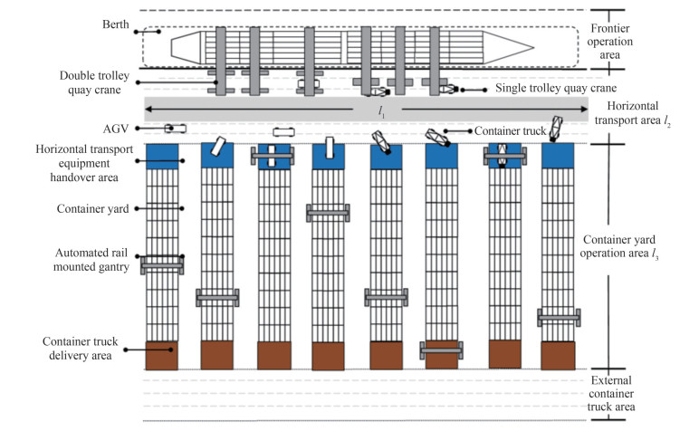Figure  1  Schematic Figure of the Automated Terminal Mixing Process

Download: Full-Size Img

The uncertainty of the speed of the horizontal transport equipment (container truck and AGV) can greatly affect the connection between the quay crane and the ARMG. Thus, the heavy and no-load speeds of the horizontal transport equipment (container truck and AGV) were considered uncertainty factors. Then, a collaborative scheduling model of automated terminal equipment resources under the hybrid process was constructed to minimize the completion time of all tasks.

3   Model building

Considering the uncertainty of the speed of the container truck and AGV, an integer programming model was established in this work to describe the mixed process problem. The following assumptions were made in this study:

1) The lifting speeds of the quay crane and the ARMG are the same when loading and unloading, the acceleration and deceleration are not considered when moving, and the speed is kept constant.

2) The power of each AGV car is sufficient, and equipment failure is not considered.

3) Loading and unloading containers are of the same sizes.

The parameters and variables of the hybrid process scheduling model are given in Table 1.

The decision variables for the hybrid process scheduling model are defined as follows:

The overall mathematical model of the hybrid process scheduling model is described as follows:

Objective function:

Eq. (1) is the overall objective function and represents the final completion time minimization. Eq. (2) is the individual container task completion time minimization, which is the subsidiary objective. Here, $ \sum\limits_{x=1}^{\text{x}}{\sum\limits_{1=1}^{\text{L}}{{{\text{t}}_{\text{xl}}}}}{{\text{y}}_{\text{xl}}}$ represents the heavy-load time of the horizontal transportation equipment (AGV, container truck), $ \sum\limits_{x=1}^{X}{\sum\limits_{{{x}^{\prime }}}^{X}{\sum\limits_{l=1}^{L}{{{Z}_{x{{x}^{\prime }}l}}}}}{{t}_{x{{x}^{\prime }}l}}$ represents the horizontal transportation equipment (AGV, container truck) no-load time, and $ \sum\limits_{x=1}^{X}{\sum\limits_{q=1}^{Q}{\sum\limits_{l=1}^{L}{{{w}_{xql}}}}}$ represents the time for horizontal transportation equipment (AGV, container truck) to wait for the quay crane (double-trolley and single-trolley quay crane).

Restrictions:

Eq. (3) indicates that a container task is transported by a single AGV, while Eq. (4) indicates the continuous operation of horizontal transportation equipment. Eqs. (5)–(6) express the relationship between the moment of the start of operation and the moment of the end of operation of the container task x on the shore bridge q, respectively. Eq. (7) represents the relationship between the moment of start of operation and the moment of end of operation of container task x on ARMG a. Eq. (8) represents the waiting time under the shore bridge when the horizontal transport equipment operates container x, while Eq. (9) represents the waiting time under the ARMG when the horizontal transport equipment operates container x. Eq. (10) ensures that the main trolley of the double-trolley quay crane is not delayed, while Eqs. (11) and (12) represent the times of AGV heavy-load and no-load, respectively. Eqs. (13) and (14) represent the time when the container truck is overloaded and unloaded, respectively. Eq. (15) represents the time constraint for the container truck to start the next delivery after completing the container task. Finally, Eq. (16) represents the time constraint for starting the next delivery once the AGV completes the container task.

4   Algorithm design

The problem studied in this paper is categorized as an NP-hard problem, which is difficult to solve with an exact algorithm. Thus, in this work, we considered the use of a heuristic algorithm to solve it. PSO has the characteristics of fast convergence speed and few parameters to be set. Thus, it is widely used in solving scheduling problems, even though its shortcomings are quite obvious. Furthermore, it can prematurely fall into the local optimum. In comparison, the SA algorithm has better searchability, which can reduce the possibility of the algorithm falling into the local optimum. Therefore, in the design of the algorithm proposed in this paper, the PSO and the SA algorithms were integrated to form the SA-PSO algorithm, which is used to solve the model.

4.1   Parameters and variables

In this paper, multilayer real-coded particles were used to represent the joint scheduling problem of hybrid processes. The coding method of the x task consists of a quay crane unloading q loads, as well as the l horizontal transport equipment carrying them horizontally and transporting them to the container area by theaARMG.

4.2   Fitness function

The present study aimed to minimize the completion time. Thus, in the SA-PSO algorithm, the objective function formula (1) is directly used as the index of the fitness function to evaluate the superiority of particles.

4.3   Initial particle design

A quality scheduling solution maximizes individual machines to perform operations; where machine conditions are the same, the number of tasks performed by each machine should be roughly homogeneous. Based on the characteristics of the scheduling problem, the optimal scheduling solution has a relatively balanced distribution of tasks, which means that the number of jobs per device should be the same. To improve the quality of the initial particles and promote the convergence speed of the algorithm in the initial stage, the tasks are randomly and evenly allocated to each quay crane, wherein each horizontal transport equipment is under the condition of ensuring randomness, as shown in Figure 2.

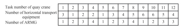Figure  2  Initial population

Download: Full-Size Img

4.4   Acceptance criteria

In the operation of quay cranes and horizontal equipment, the number of horizontal transportation equipment is greater than the number of quay cranes. As such, if the initial tasks of two quay cranes are handled by the same horizontal transportation equipment, both the quay crane and horizontal transportation equipment would be idle in the initial stage, resulting in inferior solutions. Thus, the SA algorithm is integrated to accept inferior solutions and expand the iterative search range of the PSO algorithm. Based on the above analysis, the relationship between the two algorithms, PSO and SA, was established so that the two algorithms could be integrated as follows:

● After the PSO falls into a local optimum, the optimal particle loses the ability to guide the group to find a better solution, and other particles gather toward it, losing diversity. At this time, to search for the optimal solution in the neighborhood, the SA process is initiated, and the task of a quay crane is randomly inserted into the operation sequence of another quay crane (the insertion rules for horizontal transport equipment and ARMGs are the same). If it proves to be a better solution, the previous optimal particle is replaced; otherwise, the solution is accepted according to a certain probability and expands the search range.

● As the number of iterations increases, PSO tends to fall into local convergence. In this paper, the algorithm resources were set to gradually tilt toward SA, such that when PSO was transformed to SA, the iteration stop limit of PSO was gradually assigned to SA. As a result, SA was iterated more frequently.

4.5   SA-PSO process

The specific solution steps are as follows:

Step 1: Initialize the population, set up the related parameters, and obtain the quay crane allocation plan and the order of unloading containers from each quay crane;

Step 2: According to the Metropolis criterion, calculate and normalize the fitness value of each particle at the current temperature. Then, identify the global optimal solution as follows:

Step 3: Update the speed and position using formula (17) and formula (18). Calculate the fitness value f_x and update the global optimal position x_Gb.

Step 4: Temperature judgment: if the current temperature is greater than the final temperature, go to Step 5 after cooling; otherwise, go to Step 5 directly.

Step 5: If the termination condition is satisfied, output the optimal solution; otherwise, return to Step 2.

The specific flow chart is shown in Figure 3.

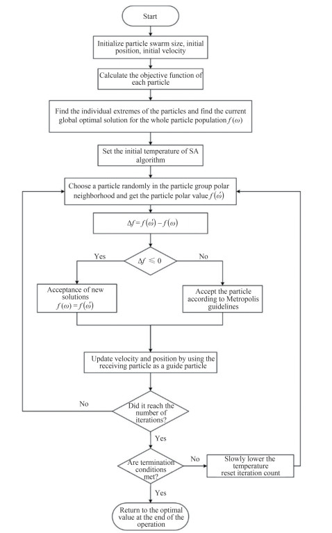Figure  3  Flow chart of the simulated annealing particle swarm optimization (SA-PSO) algorithm

Download: Full-Size Img

5   Case analysis

5.1   Study parameters

This article took the data from the Xiamen YH terminal in China as an example. There were 8 container areas in the terminal, each equipped with an ARMG. The number of container tasks was 120. Furthermore, there were three single-trolley quay cranes and three double-trolley quay cranes, which were used with six container trucks and six AGVs, respectively. The speeds of container trucks and AGVs were set as randomly generated variables within a reasonable range, where the heavy-load speed was less than the no-load speed. Based on the data of the YH terminal, the single operation time of the main and gantry trolleys of the double-trolley quay crane was set as a fixed value, and the operation time β₁ was set to 25 s. The single operation time β₃ of a single-trolley quay crane was 60 s, while the ARMG unit operation time β₄ was set to 55 s. In addition, l₁, l₂, and l₃ were the horizontal and vertical distances of the horizontal transportation area of the wharf and the distances of the yard operation area, which were 410, 674, and 236 m, respectively. We set population size N = 60, dimension D represented the number of tasks, in which the upper and lower bounds of particle position x_max were 200 and −200, respectively, the maximum speed v_max of particle movement was 400, the learning factor was 1.2, and the annealing coefficient c was 0.99. The evaluation fitness function was also generated to find the global optimal position x_Gb. The configuration of the computing environment used in the experiment is shown in Table 2, while the specific experimental parameters are shown in Table 3.

To verify the validity of the mathematical model designed for this problem, CPLEX Studio was used to transform the mathematical model to solve it. However, due to the high complexity of the problem, 30 container tasks were set to be solved. To verify the validity of the established mathe matical model, the results were also compared with those obtained from the SA-PSO algorithm proposed in this paper. The solution results are shown in Table 4.

An analysis of the solution results of CPLEX and the algorithm designed in this paper for 30 container tasks shows a deviation rate of 0.17% in absolute value, indicating that the optimal solution is similar. This means that the designed mathematical model is reasonable for the description of the operational flow of the problem.

5.2   Example solution and comparative analysis

5.2.1   Example solution

The SA PSA was used to solve the collaborative scheduling model of the hybrid process. The experiment was carried out 50 times. The optimal scheduling mode solution of the hybrid process was obtained, as shown in Figure 4 and Table 5.

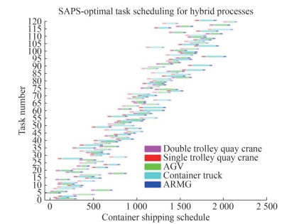Figure  4  SA-PSO for solving the mixing process scheduling

Download: Full-Size Img

Based on the calculation results, the final completion time of the optimal scheduling result of the hybrid process obtained by the SA-PSO algorithm was 2 161 s, and the "single truck quay crane + container truck + ARMG" and "two truck quay crane + AGV + ARMG" processes completed 60 containers each. The best task sequences are shown in Table 5. The solution algorithm program obtained the scheduling results within 30 s, thereby verifying the effectiveness of the algorithm we designed for this problem.

5.2.2   Comparative analysis of calculation examples

To verify the effectiveness of the hybrid process, a single loading and unloading process (single-trolley quay crane + container truck + ARMG, double-trolley quay crane + AGV + ARMG) was designed and compared with the hybrid process proposed in this paper. In the process of "single-trolley quay crane + container truck + ARMG, " 6 single-trolley quay cranes, 8 ARMGs, and 12 container trucks were set up, and the speed was randomly set within a reasonable speed range. In the process of "double-trolley quay crane + AGV + ARMG, " 6 double-trolley quay cranes, 8 ARMGs, and 12 AGVs were set up, and the speed was also randomly set within a reasonable range. The SA-PSO algorithm was used to solve the problem, and the solution results are shown in Figures 5 and 6.

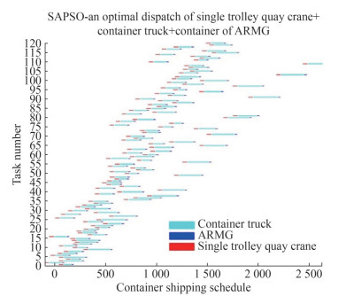Figure  5  SA-PSO algorithm to solve a single-process (single-trolley quay crane + AGV + ARMG) dispatching

Download: Full-Size Img

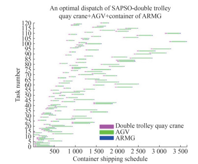Figure  6  SA-PSO algorithm to solve a single-process (double-trolley quay crane + AGV + ARMG) dispatching

Download: Full-Size Img

As shown in the analysis and calculation results in Table 6, in terms of the optimal container scheduling results obtained, the optimal scheduling time of the hybrid process is 2 161 s, and the optimal scheduling time of the "single-trolley quay crane + container truck + ARMG" is 2 620 s. The optimal scheduling time of "double-trolley quay crane + AGV + ARMG" is 3 660 s. Compared with the mixed process, the single loading and unloading processes increased by 459 s and 1 499 s, respectively, indicating that the mixed process is more effective in the same scheduling problem. This finding proves the superiority of the mixed scheduling process of the automated terminal. Second, in terms of CPU time for running and solving, the CPU time required for the hybrid process solution is 30 s, the time required for the "single-trolley quay crane + container truck + ARMG" is 80 s, and the time required for the "double-trolley quay crane + AGV + ARMG" is 130 s, the solution time of the hybrid process is greatly improved compared with that of the single process. Finally, it can be seen from the container task scheduling Gantt charts (Figures 5 and 6) that the scheduling of the hybrid process is more concentrated, the task contact is carried out, and the task arrangement is more reasonable.

5.2.3   Algorithm comparative analysis

A PSO and a GA were designed for the comparative solutions to verify the effectiveness of the proposed SA-PSA, and the data settings were the same as those of the SA-PSO algorithm.

After calculation and solution, the optimal scheduling time of the hybrid process obtained by the PSA is 2 438 s, and the CPU time for solving is 111 s. Compared with the SA-PSO algorithm, the optimal scheduling time and CPU time increased by 277 s and 81 s, respectively. Furthermore, as shown in the PSO optimal scheduling Gantt chart in Figure 7, the hybrid process scheduling scheme solved by the PSA is more scattered compared with the scheme obtained by the SA-PSO, along with greater equipment waiting time.

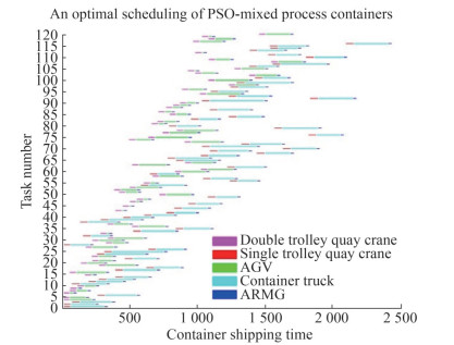Figure  7  Results of using the PSA for solving the mixing process scheduling problem

Download: Full-Size Img

The optimal scheduling time of the hybrid process obtained by selecting the enhanced elite-preserving multichromosomal GA is 2 204 s, which is 43 s longer than the optimal scheduling time of the SA-PSO algorithm. Thus, it takes a long CPU time to solve the problem using the GA. It can be seen from the optimal scheduling Gantt chart of the GA mixed process (Figure 8) that the scheduling results obtained by the GA are also more scattered compared with the scheduling results obtained by the SA-PSO algorithm. Furthermore, the equipment idle waiting time is long. Thus, in terms of the scheduling results, the performance of the device connection is not as good as that of the SA-PSO algorithm.

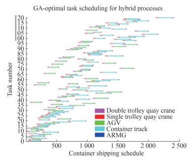Figure  8  Results of using the GA for solving the mixing process scheduling problem

Download: Full-Size Img

Figures 9 and 10 show the iterative speed of the algorithm It could be seen that the iterative convergence speed of the SA-PSO is faster, and the algorithm is more efficient. In terms of algorithm optimization, it can be seen from Figure 9 that in the initial stage of the algorithm solution, SA-PSO has strong searchability, the solution gradient descent is faster, and the optimal solution found is also better than that obtained using PSO alone.

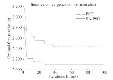Figure  9  SA-PSO and PSO algorithm iteration comparison

Download: Full-Size Img

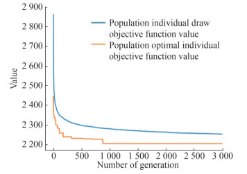Figure  10  Iterative convergence diagram of the GA Solution

Download: Full-Size Img

The iterative process of solving the problem using the GA, the most commonly used solution to solve the scheduling problem of automated container terminals, is shown in Figure 10.

As shown in Figure 10, the GA has better performance in the initial optimization and can quickly approach the approximate optimal solution. However, due to the complexity of the problem, the multichromosome real-number coding requires a considerable amount of computing resources, thus decreasing the iteration efficiency. The SA-PSO algorithm reached the approximate optimum after 40 iterations, while the GA reached the approximate optimum after 1 000 iterations. In terms of solution time, iteration times, and solution results, the SA-PSO algorithm is superior to the PSO algorithm and the GA in the areas of iterative solution efficiency and superiority of the solution obtained.

The iterative convergence speed and running results of the SA-PSO, PSO, and GA are summarized in Table 7. As shown in the table, the SA-PSO algorithm has obvious advantages compared with the traditional PSO and GA under the three algorithm performance indicators of convergence speed, CPU calculation time, and scheduling result.

6   Conclusions

In this paper, a multi-equipment resource cooperative scheduling model was constructed for automated container terminals based on a hybrid process while considering the uncertainty of the speed of container trucks and AGVs. The single loading and unloading processes were compared with the hybrid loading and unloading processes proposed in this paper. The results of the improved SA-PSO algorithm were compared with the solution results of the PSO algorithm and the GA. As such, the effectiveness of the proposed hybrid process and the improvement method were verified.

As indicated by the results, the proposed hybrid process achieved superior scheduling results by comparison. Compared with the traditional single-process, automated container terminal equipment scheduling research under traditional deterministic factors, the terminal equipment scheduling under the hybrid process, which considers the uncertain factors established in this paper, improved the overall coordination of the automated container terminal and the terminal service quality. These findings provide a reference for the improvement of the automatic terminal loading and unloading process as well as the improvement of scheduling efficiency.

In terms of limitations, the operation modes of loading and unloading were not included in the research, and there was a lack of consideration for the conflict of horizontal transportation equipment. Thus, in future research, the loading and unloading collaborative operation modes, the congestion of horizontal transportation equipment, and the uncertainty of container volume could be considered. In this way, the proposed model would be more in line with the actual operation of automated container terminals, and their operation efficiency could be effectively improved.