1   Introduction

Due to its good processing and forming properties, welding, and corrosion resistance, Q235B steel is often used as a steel for the hull structure of sea and inland river vessels. It needs to face transient physical phenomena such as stamping forming, explosion loads, and structural collisions, involving large strains (Li et al., 2020), high temperatures (Myshlyaev et al., 2010), and high strain rates (Liu et al., 2011). Therefore, the study of material deformation mechanisms at high temperatures is crucial. In a high-temperature environment, the influence of temperature and strain on the mechanical response of materials is complex and intercoupled. Numerical simulation is one of the important methods for studying dynamic responses. Constitutive models play a crucial role in describing mechanical behavior under different loading conditions. Commonly used constitutive models include the Zerilli-Armstrong model (Zerilli and Armstrong, 1987) based on physics, Arrhenius-type models (Sellars and McTegart, 1966), and Streinberg models (Steinberg et al., 1980). However, these models have complex structures, requiring a significant amount of experimentation to determine numerous parameters. Moreover, it is challenging to find material parameters in their constitutive models in publicly available literature. In contrast, the phenomenological Johnson-Cook constitutive model (Johnson, 1983), with its simple multiplicative form and accurate prediction of material deformation, is widely applied.

The Johnson-Cook constitutive model consists of two parts: the strength model representing the material's plastic flow and the failure model representing the material's fracture and failure. This paper focuses on the plastic flow part. The rheological stress in the plastic flow model is composed of three parts: strain hardening, strain rate, and temperature. Its form is well suited for finite element calculations. Scholars both domestically and internationally have concentrated their research on the numerical simulation aspects of the Johnson-Cook model. Arild H. Clausen et al, using AA5083-H116 aluminum alloy as the research object, discussed the influence of temperature, strain rate, and stress triaxiality on rheological stress and failure strain. They calibrated the Johnson-Cook constitutive model based on experimental data and explained the reason for the aluminum alloy's negative strain rate sensitivity. Wang et al. (2021) introduced a temperature term to the Johnson-Cook model, making it applicable to situations below the reference temperature. They quantitatively determined the intrinsic relationship between temperature, elastic modulus, specific heat at constant pressure, and Poisson's ratio. Huang et al. employed the downhill simplex method to establish a multi-objective function correction method with Johnson-Cook model parameters as objects. They combined simulation to correct the model parameters. Seo et al. (2022), based on tensile tests of 304 and 316 austenitic stainless steels at different strain rates, found that the effect of strain rate on stress depends not only on the strain rate but also on the plastic strain level. They proposed an improved Johnson-Cook model. Wang et al. (2020) proposed a model based on the Johnson-Cook and GTN models. Through tensile and drop hammer impact tests compared with numerical simulation results, they verified the material model and predicted the structural failure response in ship collision simulations. Zhu et al. (2021), by establishing a first-order differential model of the temperature-strain relationship, conducted finite element simulations and actual cutting experiments, improving the prediction accuracy of the modified J-C model for cutting force, cutting temperature, and chip serration. From the above research results, it is evident that research on the thermodynamic properties of metals mainly focuses on exploring optimal material constitutive models through different types of experiments to enhance the accuracy, simulation efficiency, and computational time of the models.

This paper begins by analyzing the mechanical properties of Q235B steel (Guo et al., 2022) under room temperature and high-temperature quasi-static tensile tests. The initial values of the Johnson-Cook model parameters are determined through a fitting method. Subsequently, a simulation model under room temperature is established, and the simulated mechanical performance curves for displacement and stress are monitored. Using the Poisson's ratio (u) and partial Johnson-Cook strength model parameters as design variables, the objective is set to minimize the integral of the difference between the simulation and experimental curves and the weighted error of characteristic points. Various global exploration optimization methods, such as Adaptive Response Surface, Sequential Quadratic Programming, Feasible Direction Method, Genetic Algorithm, and Global Response Surface, are employed successively to optimize and calibrate the model parameters under room temperature. The optimal algorithm for this optimization problem is determined, and sensitivity analysis is conducted to explore the impact of model parameters on the objective function. Finally, the Johnson-Cook model parameters under high temperature are calibrated using the optimal algorithm.

2   Q235B steel material performance test

Q235B low-carbon steel is widely used in ship structures, and its material composition is shown in Table 1. The stress-strain relationships of the material at normal and elevated temperatures are obtained through uniaxial tensile tests. The test specimens and test procedures are set according to GB/T 37783—2019 "Metallic materials-High-strain-rate and high-temperature tensile testing method." The test specimen is shown in Figure 1, and the 10 T Instron Universal Material Testing Machine used in the experiment is depicted in Figure 2. The high-temperature uniaxial tensile test temperature is controlled by the high and low-temperature furnace control box shown in Figure 3. When using the universal material testing machine, an extensometer is installed on the specimen to measure engineering strain e. The gauge length of the extensometer is 25 mm. Engineering stress s is calculated by dividing the force measured by the machine's pressure measuring device by the initial cross-sectional area of the specimen. Assuming material volume conservation, nominal values are converted to true values using the equations ε = ln (1 + e) and σ = s(1 + e).

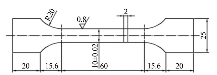Figure  1  Tensile specimen size (unit: mm)

Download: Full-Size Img

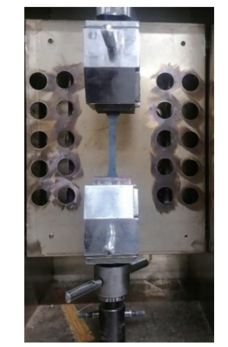Figure  2  10 T Instron universal material testing machine

Download: Full-Size Img

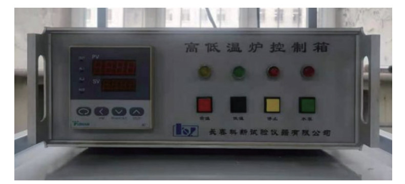Figure  3  High and low temperature furnace control box

Download: Full-Size Img

2.1   Test Ⅰ quasi-static tensile test at room temperature

The stress-strain relationship of the material at room temperature was obtained from quasi-static uniaxial tensile tests on plate specimens. Due to the good ductility of Q235B steel, the tensile speed was set to 5 mm/min, resulting in a true average strain rate of 2.1 × 10⁻¹ S⁻¹. All tests were conducted under displacement control. Figure 4 shows the true stress-strain curve at high temperatures, with the black curve representing the true stress-strain curve from quasi-static tensile tests at room temperature. It can be observed that Q235B steel exhibits a distinct yield plateau at room temperature, with a yield strength of 295 MPa.

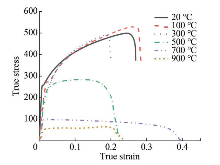Figure  4  High temperature tensile stress-strain curve

Download: Full-Size Img

2.2   Test Ⅱ quasi-static tensile test at elevated temperatures

The tensile speed for high-temperature tests was set at 5 mm/min, and the test temperatures were 20 ℃, 100 ℃, 300 ℃, 500 ℃, 700 ℃, and 900 ℃, respectively. Post-fracture photographs of specimens at high temperatures are shown in Figure 5. It can be observed that at room temperature, 100 ℃, and 300 ℃, the true stress-strain curves exhibit distinct yield plateaus. When the temperature exceeds 300 ℃, the true stress-strain curves do not show a clear yield plateau. Therefore, the yield stress at temperatures above 300 ℃ is taken as the true stress at a plastic strain of 0.02. Additionally, it is noted that there is little difference between the stress-strain curves at room temperature and 100 ℃. At temperatures of 300 ℃, 500 ℃, and 900 ℃, the fracture strain is lower than that at room temperature, and the yield stress gradually decreases with increasing temperature. At 700 ℃, the fracture strain is higher than at room temperature, but the yield stress still follows the law of decreasing with increasing temperature. It can be seen that with the change in temperature, the fracture mode also undergoes changes.

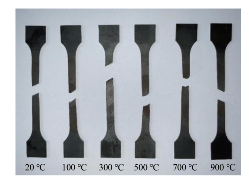Figure  5  Photo of tensile test specimen at high temperature

Download: Full-Size Img

3   Johnson-Cook strength model calibration

3.1   Johnson-Cook flow stress model

In the Johnson-Cook material model, the von Mises plasticity flow stress (σ_ep) is expressed as a function of plastic strain, strain rate, and temperature:

where $A$ is the initial yield stress, $B$ is the hardening constant, $n$ is hardening index, $C$ is the strain rate constant, $\dot{\varepsilon}_{e p}^{\mathrm{n}}$ is the equivalent plastic strain, $\dot{\varepsilon}_{e p}^*$ is the dimensionless equivalent plastic strain rate $\left(\dot{\varepsilon}_{e p}^*=\dot{\varepsilon}_{e p}/\dot{\varepsilon}_0\right.$, where $\dot{\varepsilon}_0$ is the reference strain rate), $m$ is the thermal softening index. $\sigma_{e p}$ is the equivalent flow stress, which is the product of strain hardening, strain rate, and temperature. These three factors can be individually addressed in uniaxial tensile tests, facilitating material calibration. $T^*$ is the dimensionless temperature and is defined as:

where T_r and T_m are the reference temperature and the melting temperature of the material, and T is the current temperature. The equation is valid only when T is greater than or equal to T_r.

3.2   Parameter calibration of Johnson-Cook strength model

According to test Ⅰ at room temperature quasi-static tensile. Based on the results of Experiment Ⅰ, a Levenberg-Marquardt optimization algorithm(Cao et al., 2015) was employed to fit the strength model parameters A, B, and n of Q235B steel's static tensile test at room temperature. After 8 iterations, the obtained values were A=282.4 MPa, B=537.4 MPa, n=0.575. The fitted curve and experimental curve are compared in Figure 6, with a fitting accuracy of R2 = 0.997. For Experiment Ⅱ, fitting was performed for the temperature weakening coefficient m based on the high-temperature static tensile test results. After 16 iterations, m= 0.757 was obtained. The fitted surface and experimental curve are compared in Figure 7, with a fitting accuracy of R2 =0.676. According to the fitting results, it can be observed that the model parameters for static tensile tests at the reference temperature can accurately reflect the experimental results. In contrast, due to various influencing factors in high-temperature static tensile tests, the fitting accuracy is lower, resulting in the constitutive model not accurately reflecting the material characteristics.

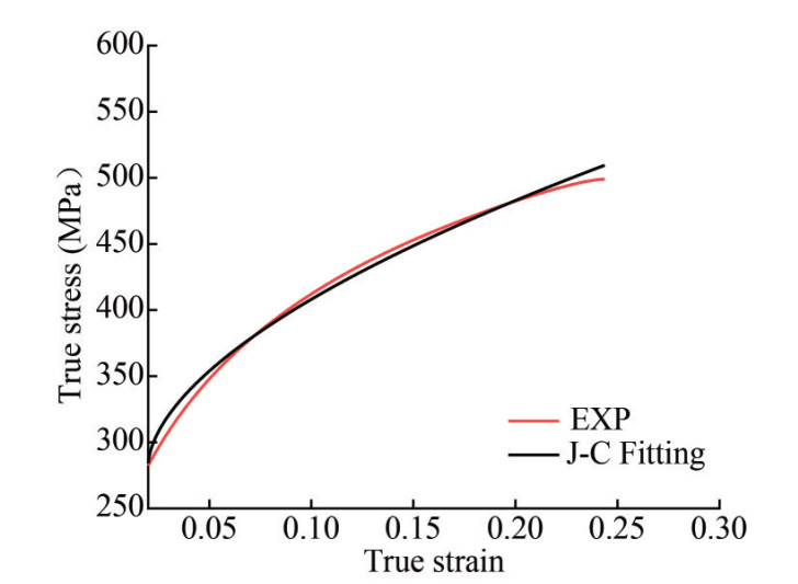Figure  6  Static stretching parameter calibration

Download: Full-Size Img

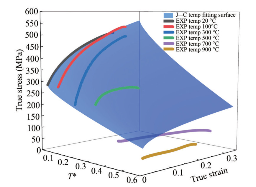Figure  7  High temperature tensile parameter calibration

Download: Full-Size Img

4   Optimal calibration of material parameters at normal temperature

The parameter calibration method mentioned above, aimed at ensuring overall accuracy, leads to significant errors in the yield stress and fracture stress compared to experimental values. The errors in yield stress and fracture stress at room temperature are 4.5% and 19.0%, respectively. Additionally, conventional calibration methods do not consider the influence of Poisson's ratio. To reduce the errors in yield stress and fracture stress, a simulation model is first established based on experimental requirements under the same conditions. The model monitors parameters such as tensile force, elongation, and cross-sectional area changes and outputs simulated stress-strain curves. Subsequently, using Poisson's ratio and Johnson-Cook strength model parameters as optimization design variables, and aiming to reduce the integral of the curve difference between the simulated and experimental curves and the weighted error between simulated and experimental values at special points as the optimization objective function, various optimization algorithms are applied to optimize and calibrate the material parameters at room temperature. The investigation explores the optimization algorithms suitable for this problem and obtains the optimal Johnson-Cook material parameters at room temperature.

4.1   Optimization model

The optimization objective for calibrating the Johnson-Cook strength model parameters at room temperature is to reduce the error between simulated yield stress, fracture stress, and experimental values. Simultaneously, it aims to ensure the error between the simulated and experimental curves, excluding two special points. For such multi-objective optimization problems, this paper linearly weights the two objective errors to transform the multi-objective optimization problem into a single-objective optimization problem.

The optimization mathematical model is as follows:

In the equation, u, A, B, n and m are the optimized design variables, and X_min and X_max represent the lower and upper bounds of the design variables, respectively. The physical definitions and limits of the design variables are provided in Table 2. This optimization model is also applicable to the subsequent optimization calibration of material parameters at high temperatures, with the main difference being the variation of design variables. The corresponding experiments for different design variables are listed in Table 2.

4.2   Optimization algorithm

For such optimization problems, the objective functions may exhibit characteristics such as multi-modality, nonlinearity, discontinuity, and non-differentiability, making it challenging to find the global optimal solution using traditional numerical optimization and direct search methods. Therefore, this study employs global exploration optimization methods such as Adaptive Response Surface Method (ARSM), Sequential Quadratic Programming (SQP), Method of Feasible Directions (MFD), Genetic Algorithm (GA), and Global Response Surface Method (GRSM) for the optimization calibration of material parameters in the quasistatic tensile constitutive model at room temperature. The iterative progress of the objective functions for different optimization methods is illustrated in Figure 8.

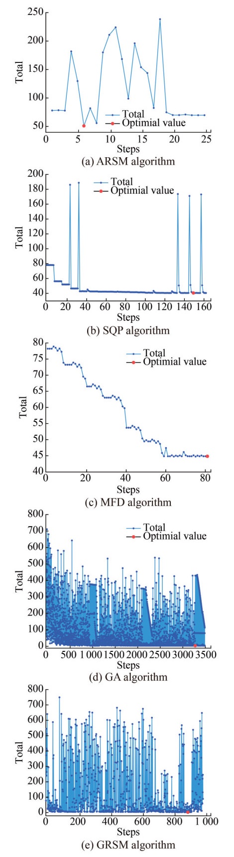Figure  8  Objective function iteration curve of different optimization algorithms

Download: Full-Size Img

It can be observed that in the initial stages, all five optimization algorithms exhibit randomness with significant fluctuations. As the number of iterations increases, they gradually converge. The optimized material parameters after using the five optimization algorithms are presented in Table 3. The optimal results of the objective functions for the first three optimization algorithms are relatively larger, while Genetic Algorithm (GA) and Global Response Surface Method (GRSM) achieve better results with objective function values of 5.025 and 3.014, respectively. Since the Global Response Surface Method (GRSM) attains the optimum in 904 steps, saving a considerable amount of computation time, it demonstrates high applicability for such optimization problems.

4.3   Analysis of optimization results

This study employs the correlation coefficient (R) and the average absolute relative error (AARE) to evaluate the model accuracy. Figure 9 presents a comparison of errors before and after optimization using different algorithms. It is evident that Genetic Algorithm (GA) and Global Response Surface Method (GRSM) yield yield and fracture values that are closer to the experimental values compared to before optimization. Moreover, the Global Response Surface Method (GRSM) achieves this with fewer iterations. Therefore, the Global Response Surface Method (GRSM) is selected as the optimization method for material parameter calibration under high temperature and high strain rate conditions in the subsequent sections.

Equations (4) and (5) represent the formulas for the correlation coefficient (R) and the average absolute relative error (AARE). Here, $N$ denotes the number of experimental data points, $E_{\mathrm{i}}$ and $P_{\mathrm{i}}$ represent the experimental and simulated data, and are the respective means of $E_{\mathrm{i}}$ and $P_{\mathrm{i}}$.

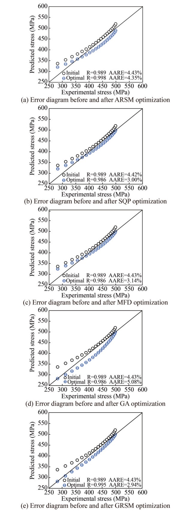Figure  9  Error diagram before and after optimization of different optimization algorithms

Download: Full-Size Img

4.4   Sensitivity analysis

The Monte Carlo method is employed for sensitivity analysis to investigate the influence of each parameter on the design variables. Utilizing a normal distribution as the probability density function, a Latin hypercube sampling method is employed for sampling to achieve the global distribution of parameters. Figure 10 illustrates the contribution rates of each design variable. It is evident that the impact of the constitutive model parameters on the shear stress is nonlinear. The initial yield stress (A), hardening constant (B), and hardening exponent (n) have a significant influence on the objective function. This is because, at room temperature, the Johnson-Cook model is directly composed of these three parameters, and their variations directly affect the objective function. On the other hand, the contribution of Poisson's ratio (u) is relatively small as its variations affect the elastic portion of the stress-strain curve indirectly. Additionally, the initial yield stress (A) and hardening constant (B) are positively correlated with the objective function, while the hardening exponent (n) and Poisson's ratio (u) are negatively correlated.

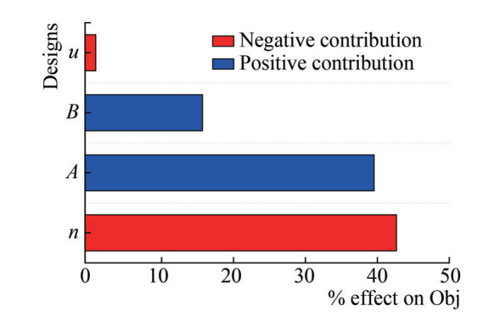Figure  10  Contribution rate of design variables

Download: Full-Size Img

5   Optimization calibration of quasi-static tensile material parameters at high temperature

Firstly, the environmental temperature is set according to the requirements of high-temperature tests, and the design variables for the optimization and calibration of material parameters under high temperature include an additional thermal softening index (m) compared to room temperature. As temperature variations can affect the Poisson's ratio, when optimizing and calibrating material parameters under high temperature, the Poisson's ratio at each temperature is selected as a separate design variable to explore its variation with temperature. The initial values and optimization ranges of other design variables remain consistent with those at room temperature. The objective function is set as the linear weighted sum of the objective function at six temperatures, and the global response surface algorithm is used to find the optimal parameter combination. The optimization objective function involves the linear weighted sum of the integral of the curve difference between simulated and experimental values and the error of characteristic points for each temperature range. Figure 11 illustrates the iteration curve of the objective function during high-temperature quasi-static tensile testing. The red point represents the optimal solution of the objective function, reached in 616 steps. The green points represent local optimal solutions for each temperature, reached at 625, 364, 637, 615, 603, and 320 steps, respectively. The optimal Poisson's ratios at six temperatures are 0.249, 0.291, 0.348, 0.311, 0.325, and 0.367, respectively. It can be observed that the Poisson's ratio generally increases with temperature, further confirming that introducing the Poisson's ratio at different temperatures as design variables has a certain effect on reducing the objective function. After optimization, the values of the Johnson-Cook model parameters are A= 187.4, B=710.6, n=0.431, and m=0.573.

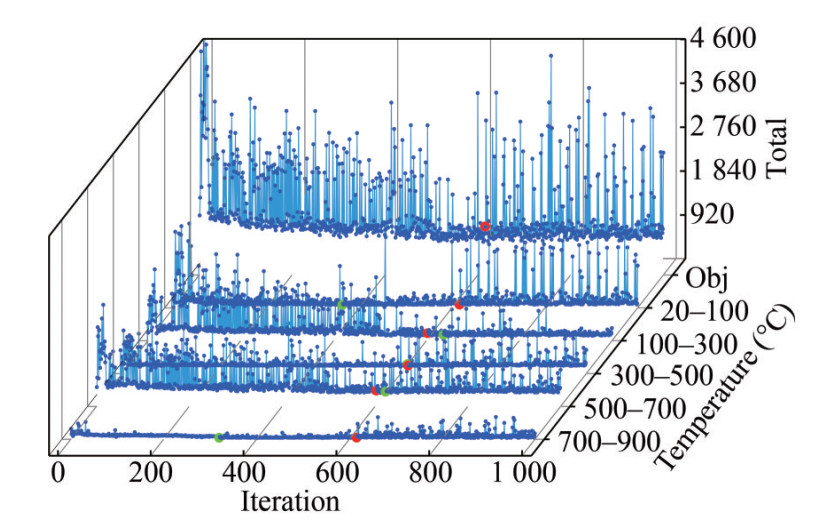Figure  11  Iterative curve of quasi-static tensile objective function at high temperature

Download: Full-Size Img

Table 4 shows the changes in relevant parameters before and after optimization at different temperatures. It can be observed that, similar to the optimization results at room temperature, the correlation coefficient exhibits a decreasing trend, and the average relative error shows an increasing trend, indicating an overall increase in the error of the simulated curve after optimization. However, the objective function at each temperature decreases, aligning with the optimization design goal and confirming that the global response surface algorithm is equally applicable to the optimization and calibration of material parameters under high temperature. Additionally, the reduction in the objective function is mainly attributed to the decrease in errors of the yield stress and fracture stress. This phenomenon arises because the error values of the characteristic points are slightly higher than the curve integral values, contributing more to the objective function. Even if the curve integral increases, it can be offset as long as the error in the characteristic points decreases.

6   Conclusions

This study investigates the mechanical properties of Q235B steel through quasi-static tests at both room temperature and elevated temperature. The initial values of the Johnson-Cook model parameters are determined using a fitting method. Subsequently, a simulation model is established, and the mechanical performance curves for displacement and stress are monitored. Taking Poisson's ratio (u) and the Johnson-Cook model parameters as design variables, the objective function is defined as the weighted sum of the integral of the difference between simulation and experimental curves and the error of characteristic points, aiming to minimize this function. The global response surface algorithm is employed to optimize and calibrate the Johnson-Cook model parameters for Q235B steel under both room temperature and elevated temperature conditions. The conclusions obtained are as follows:

The global response surface algorithm is more suitable for material parameter optimization and calibration compared to the adaptive response surface algorithm, sequential quadratic programming, feasible direction method, and genetic algorithm. The optimal parameters for the model under room temperature obtained through optimization are as follows: u= 0.284, A=173.5, B=621.6, n=0.387.

Through sensitivity analysis, the influence of model parameters on the objective function was explored, revealing that the initial yield stress (A), hardening constant (B), and hardening exponent (n) have a significant impact on the objective function. The initial yield stress (A) and hardening constant (B) are positively correlated with the objective function, while the hardening exponent (n) and Poisson's ratio (u) are negatively correlated with the objective function.

Using the global response surface algorithm for the optimization calibration of model parameters at high temperatures, introducing the thermal softening index (m) and Poisson's ratios at different temperatures as design variables, the iteration process yields the variation of Poisson's ratios with temperature and the optimal parameters at high temperatures as follows: A=187.4, B=710.6, n=0.431, m=0.573.

From the optimization calibration results, it can be observed that the objective functions at both room temperature and high temperature are reduced compared to before optimization. The values of yield stress and fracture stress are also closer to experimental results, indicating that the material strain mechanisms over a wide temperature range align more closely with actual experimental results.

From the analysis results, it can be observed that the reduction in the objective function is mainly attributed to the decrease in yield stress and fracture stress errors. The integral of the curve difference has a relatively small magnitude and has little impact on the objective function. Therefore, future work could involve analyzing the influence of different weight combinations on the optimization convergence speed and accuracy.