1   Introduction

Channel estimation plays a crucial role in underwater acoustic (UWA) communication. In terms of implementation, existing methods can be categorized into two classes: frequency-domain and time-domain approaches. The frequency-domain class (Wang and Dong, 2006; Zheng et al., 2010) involves the design of specific frame structures, such as the dual Unique Word (UW) design in a single-carrier frequency-domain equalization (SC-FDE) system, which transform the channel matrix into a diagonal matrix in the frequency domain. While these methods are relatively simple to implement and have low complexity, their applicability and performance are limited in certain scenarios. Alternatively, time-domain techniques have emerged as the dominant approach in channel estimation due to their flexibility and accuracy. These techniques allow estimation using training sequences without any additional constraints. Among them, estimators based on the least square (LS) (Coleri et al., 2002) and minimum mean square error (MMSE) (Kang et al., 2003) criteria are widely used. However, their performance is also constrained without consideration for the sparsity of the UWA channel.

Compressive sensing is a crucial technique in sparse channel estimation, covering greedy methods (Panayirci et al., 2019; Wang et al., 2021), norm-constrained approaches (Li et al., 2016; Tsai et al., 2018; Wu et al., 2013), and Bayesian methods. Among them, sparse Bayesian learning (SBL) holds particular importance within the Bayesian framework. It was initially introduced in (Tipping and Michael, 2001) and subsequently applied to UWA channel estimation in (Cho, 2022; Feng et al., 2023; Jia et al., 2022). It was based on a linear model, employed a hierarchical probability distribution, and iteratively solved the posterior expectation of the channel vector. So far, the SBL has been further developed in various scenarios. A block-based SBL (BSBL) was presented in (Zhang and Rao, 2011), which further considered the temporal correlation of measurement vectors. Additionally, a joint SBL (JSBL) was proposed to enable joint channel and data detection in quasi-static channels in (Prasad et al., 2014), and then a Kalman filtering-based SBL (KSBL) was derived for time-varying cases that adopted a first-order autoregressive model.

The classical sparse Bayesian learning (SBL) was derived using the expectation maximization (EM) algorithm (Tipping and Michael, 2001). It estimated the hidden variable through maximum likelihood or maximum a posteriori estimation. However, even after convergence, there was still a discrepancy between the estimated value and the real posterior expectation. Additionally, the aforementioned optimization-based SBL algorithm cannot address this issue. Therefore, we introduce a SBL method that incorporates variational inference (Ⅵ) (Zhang et al., 2018) and Markov chain Monte Carlo (MCMC) (Casella and George, 1992) to enhance the estimation accuracy of the UWA channel.

The Ⅵ is a method that infers hidden variables by approximating their posterior distribution with a simpler variational distribution. It is noted that the EM algorithm is a special instance of Ⅵ when the posterior distribution of the hidden variables is known. Thereby, the SBL can also be approximately derived from Ⅵ. Although the formulas for EM and Ⅵ yield identical results, they carry different physical interpretations. On the other hand, MCMC is also an inference method that allows random sampling from a given analytic posterior distribution. It constructs a Markov chain that converges to a smooth distribution consistent with the target posterior distribution. In comparison to EM and Ⅵ, MCMC often demonstrates better performance. Gibbs sampling is an efficient implementation of the MCMC method, the performance of which in various scenarios has been further analyzed and developed. In previous work (Gelfand and Lee, 1993), a summary of some preliminary findings regarding the computational burden under various implementations of the Gibbs sampler is provided. The results reveal that the Metropolis-within-Gibbs method appears to be superior and exhibits less runtime compared to the other methods in both provided cases. Another study (Goudie and Mukherjee, 2016) presented a Gibbs sampler for learning the structure of directed acyclic graph (DAG) models. In contrast to the standard Metropolis-Hastings sampler, it draws complete sets of parents for multiple nodes from appropriate conditional distributions, providing an efficient method for making large moves in graph space, allowing faster mixing while retaining asymptotic guarantees of convergence. Recently, in a work by Martino et al. (2018), it is shown that the auxiliary samples can be recycled in the Gibbs estimator, thus increasing efficiency without additional cost. This advancement has the potential to improve the overall performance of Gibbs sampling.

In this study, we first derive SBL based on Ⅵ, approximating the posterior distribution of the channel, hyperparameters, and noise variance. Subsequently, we substitute the real posterior distribution with the variational distribution and determine the full conditional probability distributions for various variables. Finally, random Gibbs sampling in MCMC is efficiently performed to guarantee the convergence of Markov chain. The results of simulation and experiment demonstrated that compared to the classical SBL approach, the channel impulse response could be reconstructed more effectively.

This paper is organized as follows. Section 2 describes the model for UWA channel estimation and SBL; Section 3 details the Gibbs sampling-based sparse channel estimation method; the results of simulation and experiment are shown in Section 4 and Section 5, respectively. Finally, Section 6 concludes the whole paper.

2   System model

Consider a single-input single-output (SISO) UWA single-carrier communication system. The original binary bits are encoded, interleaved and mapped to produce the transmitted vector x = [x₁, x₂, …, x_N]^T ∈ C^{N × 1}, where N is the number of symbols and (•)^T indicates the transpose operation. Suppose the baseband length of the UWA channel is L and the observed length is M. The model for channel estimation at the receiver can be expressed as

where y = [y₁, y₂, …, y_M]^T ∈ C^{M × 1} denotes the observed vector and n = [n₁, n₂, …, n_M]^T ∈ C^{M × 1} represents the noise vector with mean of zero and variance of σ².

In SBL, the element h_l of the channel vector h = [h₁, h₂, …, h_L]^T ∈ C^{L × 1} to be estimated is assumed to be independent and identically distributed (i.i.d.), which is adjusted by corresponding element α_l in hyperparameter vector α = [α₁, α₂, …, α_L]^T ∈ C^{L × 1}. The probability distribution can be expressed as

where $\mathcal{C N}$ denotes the complex Gaussian distribution. In addition, both α⁻¹ and σ⁻² are assumed to obey the prior distribution of Gamma, satisfying

The $\mathcal{G}$ denotes the Gamma distribution with a, b, c and d being known parameters. Meanwhile, the likelihood function in Eq. (1) obeys an M-dimensional independent complex Gaussian distribution, i.e.,

where ‖•‖₂ represents the 2-norm of a vector. To date, the probability model of SBL in UWA channel estimation has been built. According to Eqs. (3)‒(6), the joint distribution of all variables can be expressed as

3   Gibbs sampling-based sparse channel estimation method

In this section, the SBL will first be re-derived through Ⅵ. In Eq. (7), the unknown h, α⁻¹, σ⁻² together form the set of hidden variables Ω ={h, α⁻¹, σ⁻²}. Accordingly, we can define the mean-field variational distribution q_Ω (Ω)= q_h (h)q_α⁻¹ (α⁻¹)q_σ^-2 (σ⁻²). The idea of Ⅵ lies in minimizing

where $\mathcal{K L}$ refers to the divergence and p (Ω | y) is the real posterior distribution. This objective can be achieved by updating each variational factor in turn (Zhang et al. 2018), as summarized in Eqs. (9)‒(11).

Bringing Eqs. (2)‒(6) into Eqs. (9)‒(11), it is obtained that q_h (h) follows the complex Gaussian distribution, as well as q_α⁻¹ (α⁻¹) and q_σ⁻² (σ⁻²) obey the Gamma distribution,

where (•)^H stands for the conjugate transpose and tr (•) represents the trace of a matrix. The μ_{h, i} and Σ_{h, i} is the ith element of μ_h and the ith diagonal element of Σ_h respectively.

Here μ_σ⁻² is the mean of distribution q_σ⁻² (σ⁻²) and A is a diagonal array consisting of the mean μ_αl⁻¹ of distribution q_α⁻¹ (α⁻¹),

Eqs. (12)‒(19) exhibit the results of approximating the SBL with the variational distribution. Depending on Gibbs sampling (Casella and George, 1992), when starting from an initial sample Ω₀ ={h⁽⁰⁾, α^{−1, (0)}, σ^{−2, (0)}} of the target distribution p (Ω | y), and sequentially sampling the full conditional probability distributions p (h | y, α^{−1, (i−1)}, σ^{−2, (i−1)}), p (α⁻¹| y, h⁽ⁱ⁾, σ^{−2, (i−1)}), and p (σ⁻²| y, h⁽ⁱ⁾, α^{−1, (i)}) with respect to variables h, α⁻¹, σ⁻², we construct a randomly wandering Markov chain with its smooth distribution corresponding to p (Ω | y). The Ω_i ={h⁽ⁱ⁾, α^{−1, (i)}, σ^{−2, (i)}} denotes the ith finished sample of hidden variables, and x⁽ⁱ⁾ indicates the ith sample value of x.

As Ⅵ minimizes the $\mathcal{K L}$ divergence between q_Ω (Ω) and p (Ω | y), accordingly, we can sample from q_Ω (Ω) instead of p (Ω | y). Thus, the full conditional probability distributions of h, α⁻¹, σ⁻² are now expressed as

In Eqs. (20) ‒ (21) and (22), we begin by dividing the joint variational distribution q_Ω (Ω) by the prior variational distributions of the irrelevant variables, yielding the conditional distributions of the target variable. Next, we determine the full conditional probability distribution of by incorporating the current values of the remaining variables.

For instance, in the ith iteration, we first compute the full conditional probability distribution of the channel. Since $q_{\Omega}(\Omega)=q_{\boldsymbol{h}}(\boldsymbol{h}) q_{\boldsymbol{\alpha}^{-1}}\left(\boldsymbol{\alpha}^{-1}\right) q_{\sigma^{-2}}\left(\sigma^{-2}\right)$ and the current values of hyperparameters and noise variance are from the (i − 1) iteration, the result on the first side of Eq. (20) is equal to $q_{\boldsymbol{\alpha}^{-1}}\left(\boldsymbol{\alpha}^{-1} \mid \boldsymbol{h}^{(i)}, \sigma^{-2, (i-1)}\right) $. Then simply sample from q_h(h|α^{−1, (i−1)}, σ^{−2, (i − 1)}), $q_{\boldsymbol{\alpha}^{-1}}\left(\boldsymbol{\alpha}^{-1} \mid \boldsymbol{h}^{(i)}, \sigma^{-2, (i-1)}\right)$ and $q_{\sigma^{-2}}\left(\sigma^{-2} \mid \boldsymbol{h}^{(i)}, \boldsymbol{\alpha}^{-1, (i)}\right)$ in turn, satisfying

where

The A⁽ⁱ⁻¹⁾ is composed of the sampled values of the hyperparameters at this point,

Besides, $q_{\boldsymbol{\alpha}^{-1}}\left(\boldsymbol{\alpha}^{-1} \mid \boldsymbol{h}^{(i)}, \sigma^{-2, (i-1)}\right)$ and $q_{\sigma^{-2}}\left(\sigma^{-2} \mid \boldsymbol{h}^{(i)}, \boldsymbol{\alpha}^{-1, (i)}\right)$ satisfy

Assume that the total iterations of the method are I and the times consumed before the Markov chain reaches smooth distribution are P. The final estimated value of UWA channel is

Define x⁽ⁱ⁾ ~p (x) to be sampling from the distribution p (x) in the ith iteration. The procedure of the Gibbs sampling-based channel estimation method is summarized in Algorithm 1:

4   Simulation results

In this section, we evaluated the performance using the SC-FDE system. The simulation was conducted in baseband, employing a block length of 512 symbols (N = 512). The simulated channel, illustrated in Figure 1, consisted of L = 48 taps. In the subsequent analysis, the parameters c and d were set to 0, while a was 1 and b was 0.000 1 to ensure a relatively large variance for the channel. We set the number of iterations to 500 for both the SBL and our proposed method. Additionally, we adopted the Gibbs sampling method with P = 200, which utilized the last 300 samples to estimate the expectation of the channel.

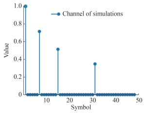Figure  1  UWA channel of simulations

Download: Full-Size Img

Figures 2‒4 displayed the comparison between the SBL and the proposed channel estimation method in terms of mean square error (MSE) and bit error rate (BER) with varying observed length M. For the BER simulation, we uniformly used the MMSE equalizer. The dashed line in the figure indicated the simulation results obtained with an ideal channel. As shown in Figures 2(a), 3(a), and 4(a), the Gibbs sampling-based approach outperformed SBL at various signal-to-noise ratios (SNRs), especially at lower M. According to Figures 2(b), 3(b) and 4(b), it also better reduced the BERs of the system. When M was 276 and the SNR was 8 dB, the gap with the system using ideal channel was less than 0.2 dB, which proved the effectiveness of the method.

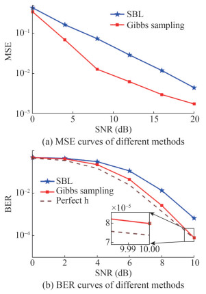Figure  2  Simulation performance with M = 76

Download: Full-Size Img

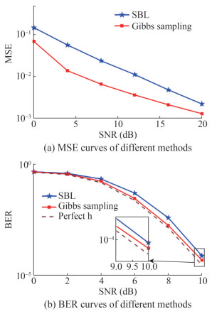Figure  3  Simulation performance with M = 176

Download: Full-Size Img

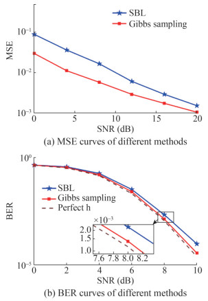Figure  4  Simulation performance with M = 276

Download: Full-Size Img

To analyze the convergence of Markov chains during Gibbs sampling, we took the MSE of channel expectation in neighboring iterations as a measure, defined as Q, satisfying

Figure 5 exampled the convergence for varying M and SNRs. When the value of Q stabilized near zero, it indicated that the Markov chain had achieved a steady distribution. Then, sampling could be performed on the posterior distribution of the channel to compute the expectation.

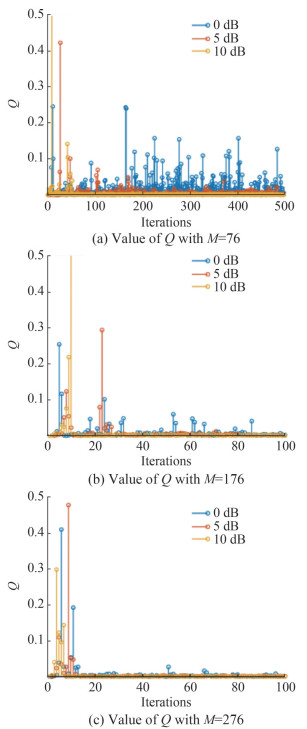Figure  5  Comparison of convergence with Gibbs sampling under different M and SNR

Download: Full-Size Img

The results revealed that the Markov chain converged more rapidly as the observed length M increased at the same SNR. For instance, at 0 dB, convergence was not achieved within 500 iterations for M = 76, while it typically converged within 100 iterations for M = 276. Similarly, for the same observed length, faster convergence was observed at higher SNRs. When the SNR was 10 dB and M = 76, our method converged within 100 iterations, and for M = 176 or 276, convergence was achieved within 20 iterations.

As depicted in Figure 6, the Gibbs sampling method is capable of converging within 50 iterations at an observed length of 76. As the observed length increases, the convergence is further accelerated, and the amplitude of fluctuations decreases. Although it may have a relatively slower convergence rate compared to SBL, it is still considered acceptable.

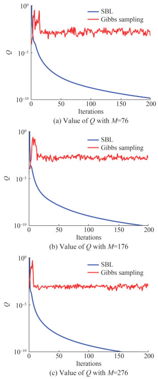Figure  6  Comparison of convergence with two methods under different M

Download: Full-Size Img

It is important to highlight that our main focus should be on the convergence speed of the two methods rather than the specific Q values they ultimately converge to. The convergence values primarily serve as an indicator of the convergence speed and not the estimated performance, which should be evaluated based on the results of MSE presented in Figures 2‒4. When the Gibbs sampling approach is employed, the channel undergoes updates along with samples of hyperparameters and noise variance during the iterative process by Equations (24) and (25). Therefore, the mean of the channel will also experience fluctuations around the real value. Once the magnitude of these fluctuations stabilizes, we can consider the Markov chain to have reached a stabilized state, and then use the smoothed samples to estimate the channel. In contrast, there is no random sampling process in the SBL method, which directly employs the EM algorithm to update the channel, ensuring that each iteration tends to converge with a diminishing Q value.

5   Experimental results

The algorithms were evaluated using data collected from an offshore UWA experiment carried out in the Yellow Sea in April 2022. The average water depth during the experiment was approximately 20 m. In this experiment, four hydrophones were deployed at fixed positions underwater, ranging from 3 to 7.5 meters deep at the receiver location. The transmitter ship was positioned at various distances to transmit signals using a SC-FDE system. The specific parameters used in the experiment are presented in Table 1.

Figures 7 and 8 illustrated the time-frequency and channel characteristics of a received frame at distances of 800 m and 3 km, respectively. In Figures 7(a) and 8(a), each frame consisted of 5 data blocks and two linear frequency modulated (LFM) signals with a duration of 500 ms, which were utilized for Doppler compensation. Analysis of Figures 7(b) and 8(b) revealed that the Gibbs sampling-based method closely approximates the SBL for the main channel taps, while exhibiting greater suppression for taps with smaller amplitudes. Consequently, as the channel sparsity increases, the method’s advantages are expected to become more pronounced.

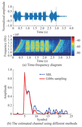Figure  7  The received waveform and UWA channel at 800 m

Download: Full-Size Img

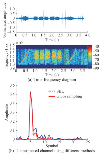Figure  8  The received waveform and UWA channel at 3 km

Download: Full-Size Img

For the experiment, we transmitted 15 frames of signals at distances of 800 m and 3 km, respectively. In total, 30 frames, equivalent to 150 data blocks, were collected. The comparison of BER using SBL and Gibbs sampling was presented in Figure 9, with the adoption of the MMSE equalizer. At a distance of 800 m, the BER obtained with SBL was 7.83×10⁻³, while the Gibbs sampling-based method achieved a lower BER of 5.56×10⁻³. Similarly, at 3 km, the BER values were 6.19×10⁻³ for SBL and 5.46×10⁻³ for the Gibbs sampling-based method. These results confirm that the Gibbs sampling-based approach is capable of more efficient reconstruction of sparse channels, leading to improved BER performance.

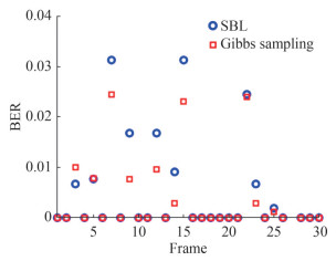Figure  9  The BER comparison using SBL and Gibbs sampling

Download: Full-Size Img

6   Conclusion

In conclusion, we presented a Gibbs sampling-based method for sparse UWA channel estimation. Our method utilized variational distributions to approximate the real posterior distribution of the channel and performed random sampling. It demonstrated superior performance compared to the classical SBL approach. Through extensive simulations, our method achieved lower MSE and BER across different observed lengths. Specifically, at an observed length of 276 and an SNR of 8 dB, the performance gap with the ideal channel was less than 0.2 dB, highlighting its effectiveness. Moreover, our method exhibited faster convergence within 20 iterations for observed lengths greater than 176 and an SNR of 10 dB. Experimental results from the Yellow Sea further supported the superiority of our method, showing lower BER at distances of 800 m and 3 km compared to SBL.