1   Introduction

In the field of array signal processing (Zhang et al., 2020; Sheng et al., 2023; Lu, 2023), beamforming techniques have been playing a key role in underwater acoustic engineering. Among the beamforming algorithms, the conventional beamforming (CBF) has been widely applied in underwater acoustic array signal processing because of its robustness against signal mismatch, and it requires only a few data snapshots to achieve a reliable estimation of target angles. However, CBF still has some disadvantages, such as the wide mainlobe (making it difficult to detect two neighboring targets of equal strength) and the high sidelobe level (making it difficult to detect weak targets with loud interference).

The decomposition of the received wideband data into many narrowband data or nonoverlapping band-pass filter banks in the frequency domain, followed by the existing narrowband beamforming algorithms, is an intuitive method of wideband signal processing. Among the beamforming algorithms, the easiest way to process wideband signals is the incoherent signal subspace method (ISSM) (Zhang et al., 2010; Ahmad et al., 2018), and the output beam power can be obtained using the average of all frequency sub-bands. Although ISSM can be applicable at different SNRs, its overall performance is inferior because of its poor beamforming at certain frequency bands (Hu et al., 2018). Subsequently, the coherent signal subspace method (CSSM) is utilized to obtain a set of narrowband signals via multiple narrowband filter banks in the frequency domain (Wang and Kaveh, 1985; Chen and Zhao, 2005; Li et al., 2018). For a specified angle, CSSM aligns the array flow patterns of each frequency dot to a uniform array flow pattern at the focusing frequency. Referring to a previous study (Swingler and Krolik, 1989), the estimation deviation of the CSSM method increases with the increase in bandwidth. Moreover, the output SNR changes after the focusing transform. By contrast, the SNR does not suffer a loss by the unitary focusing transform. Thus, Hung and Kaveh (1988) proposed the rotational signal subspace (RSS) method, which designs the unitary focusing transform matrix by presetting the steering vector of the target angle. Ma and Zhang (2019) introduced a method that can minimize the focusing transform error. Sellone (2006) proposed a robust CSSM (R-CSM) -based focusing transform that does not require prior knowledge of target angles and decreases the focusing transform error by iteratively narrowing the bearing interval between targets. Furthermore, the iterative process results in a significant increase in the calculation amount.

Yang(2017, 2018) applied the deconvolution method to CBF and proposed a deconvolved CBF algorithm that can reduce the mainlobe width, lowers the sidelobe level, and retains the robustness of CBF (Bahr and Cattafesta, 2012). Recently, global experts have focused considerable attention on the actual application of deconvolution beamforming algorithms, such as uniform acoustic pressure array (Xenaki et al., 2012), uniform circular array (Tiana-Roig and Jacobsen, 2013), vector array (Sun et al., 2019), and acoustic image measurement (Mei, 2020). As a result, the advantages of the deconvolution beamforming algorithm, such as high bearing resolution, low sidelobe level, and robustness, have been verified.

Therefore, for wideband CBF, by combining focusing transform with deconvolution, a focused-and-deconvolved beamforming algorithm is proposed. First, wideband CBF is converted into narrowband CBF at the focusing frequency by the focusing transform. Then, a high-resolution beam power is achieved, deconvolving the wideband beam power. As a result, the focused-and-deconvolved beam power is confirmed to yield a narrower mainlobe and lower sidelobe level and retain the robustness of wideband CBF.

The outline of this paper is organized as follows: First, Section 2 introduces the basic principle, which is composed of three parts: (a) signal modeling; (b) the focusing transform methods, i.e., RSS and R-CSM; and (c) the Richardson–Lucy (R-L) iterative algorithm. Then, Section 3 presents the numerical simulation results of the output beam power, the high bearing resolution, and the anti-noise performance. Subsequently, using the sea trial data processing results, Section 4 sufficiently verifies the feasibility of the proposed algorithm. Finally, Section 5 provides the conclusion of this paper.

2   Basic principle

2.1   Signal modeling

Assuming that, under far-field conditions, an N-sensor uniform linear array (ULA) is utilized for direction finding. With the frequency band [f_L, f_H] divided into J sub-bands, the array output of the j^th sub-band is derived as follows:

where f_j is the center frequency of the j^th sub-band, A(f_j) is the array flow pattern, S (f_j) is the source signal, and N (f_j) is the Gaussian white noise, uncorrelated to the source.

First, the focusing transform matrix T (f_j) satisfies the Eq. (4) as follows:

where T (f_j) is the focusing transform matrix of the j^th sub-band, f₀ is the focusing frequency dot, and A(f₀) is the array flow pattern.

Then, the array output X (f_j) is preprocessed by the formulated T (f_j), and the processing results are expressed as follows:

Subsequently, the CM of the received data is the sum and average of the CMs of all sub-bands, expressed as follows:

Finally, the focused output beam power is derived as follows:

where W (θ) = [ω₁(θ), ω₂(θ), …, ω_N(θ)]^H.

2.2   RSS-based focusing transform

In this subsection, the optimal focusing transform matrix is formulated based on the minimum error criterion, expressed as follows:

where θ is the scanning angle; A(f_j, θ) and A(f₀, θ) are the array flow patterns of the j^th sub-band and the focusing frequency, respectively; I is a J × J identity matrix.

The output beam power of the focused CBF (F-CBF) can be obtained by substituting T (f_j) into Eqs. (4) and (5).

2.3   R-CSM-based focusing transform

Based on the RSS-based method, the output beam power, with prior knowledge of target angles, is obtained. However, in practice, it is infeasible for real-time data processing. Thus, a novel focusing transform method without prior knowledge of target angles, i. e., the R-CSM method, is adopted.

where u = sin θ/2 is the scanning angle in sine form; A(u, f_j) and A(u, f₀) are the array flow patterns of the j^th sub-band and the focusing frequency, respectively; and I is a J × J identity matrix.

Based on the R-CSM-based method, the output beam power of the robust focused conventional beamforming (RF-CBF) can be obtained by substituting T(f_j) into Eqs. (4) and (5).

2.4   R-L iterative algorithm

Based on the maximum likelihood of the Bayesian theory (Richardson, 1972), the R-L iterative algorithm was proposed by Richardson and Lucy. A blurred image is deconvolved by a given point scattering function (PSF) according to the statistical criterion of Poisson noise. After a certain iteration number, the maximum likelihood estimation with high accuracy is obtained. Then, the relevant formula derivation (Ströhl and Kaminski, 2015; Ma et al., 2020) is briefly introduced.

Let us consider there exists a source signal s (x) that spreads through a channel whose impulse response function is h (y|x). If n (y) is the isotropic noise, then the received signal r (y) can be written as follows:

Deconvolution is used to restore the source signal from the received data, given that the CIR is known. Assuming that both the received data and the CIR are positive definite functions, the source signal is restored using the R-L iterative algorithm as follows:

where both $r^{(i)}(y)=\int\limits_{-\infty}^{+\infty} h(y \mid x) s^{(i)}(x) \mathrm{d} x$ and s⁽ⁱ⁾(x) converge to a unique solution after I iterations, expressed as follows:

where L (·) is Csiszar’s discrimination, which can be expressed as follows:

where h (y|x) is regarded as the PSF and assumed to be shift-invariant and can be expressed as follows:

The output beam power of CBF is regarded as the convolution between the array directivity pattern and the angle–amplitude distribution function of the sources. Thus, Eq. (5) is rewritten as follows:

Given that the PSF is known, the angle–amplitude distribution function of the sources can be obtained by deconvolving the CBF beam power B_CBF.

2.5   Procedures of the focused-and-deconvolved method

Eqs. (10) and (13) show that the output beam power of F-CBF and RF-CBF can be separately deconvolved by the R-L iterative algorithm. Therefore, as shown in Figure 1, two focused-and-deconvolved beamforming algorithms are proposed, i.e., FD-CBF and RFD-CBF.

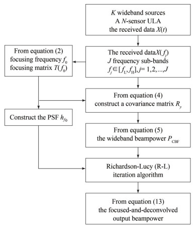Figure  1  Diagram of the focused-and-deconvolved method

Download: Full-Size Img

3   Numerical simulation

A 32-element half-wavelength spaced ULA is used to receive data. The target with an SNR of 25 dB consists of 50 consecutive 0.2 s chirp signals and arrives at the direction of arrival (DOA) of 30°. The ambient noise is Gaussian white noise, which is uncorrelated to the target. The operating frequency band ranges from 900 to 1 000 Hz. Notation: the sampling rate is 32 kHz; the focusing frequency is 1 kHz; the beam power is plotted in sine form; the observation angle measured from the broadside of the ULA ranges from −90° to 90°.

3.1   Output beam power

Figure 2(a) shows the output beam power of FD-CBF compared with that of the RSS-based focusing transform, and Figure 2(b) shows the output beam power of RFD-CBF compared with that of the R-CSM-based focusing transform. The focused-and-deconvolved beam power has a narrower mainlobe and lower sidelobe level compared with the CBF beam power. Moreover, the background level of the focused-and-deconvolved beam power (FD-CBF and RFD-CBF) is 3 dB lower than those of conventional beam power (CBF) and focused beam power (F-CBF and RF-CBF).

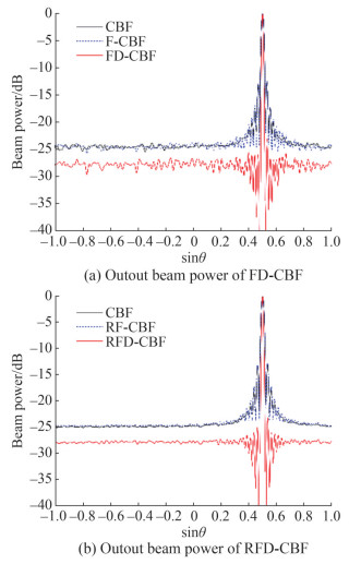Figure  2  Output beam power

Download: Full-Size Img

Subsequently, the focused-and-deconvolved output beam power (FD-CBF and RFD-CBF) is analyzed by conducting 100 Monte Carlo trials of the mainlobe width, first sidelobe level, and root–mean–square error (RMSE).

3.1.1   Mainlobe width

Here, the mainlobe width is defined as the bearing interval between the first zero points of both sides of the main beam (Farina, 2002). For one target at 0°, the mainlobe width is analyzed with the number of elements ranging from 10 to 90. The other parameters are kept constant.

Figure 3 shows that the mainlobe width decreases with the increase in the number of elements. The mainlobe widths of CBF, F-CBF, and RF-CBF are close to each other, indicating that the focusing transform does not influence the mainlobe width. Furthermore, the mainlobe widths of FD-CBF and RFD-CBF become narrower. When the number of elements is 10, the mainlobe width of RFD-CBF is wider than that of FD-CBF. When the number of elements reaches 60 or more, the mainlobe width curves of FD-CBF and RFD-CBF coincide. Thus, we have proven that the focused-and-deconvolved method can narrow the mainlobe width.

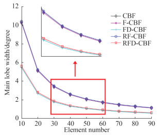Figure  3  Mainlobe width

Download: Full-Size Img

3.1.2   First sidelobe level

For one target at 0°, the first sidelobe level is evaluated with the number of elements increasing. The other parameters are kept constant.

Figure 4 shows that the first sidelobe level decreases with the increase in the number of elements. With the number of elements increasing from 10 to 90, the first sidelobe levels of CBF, F-CBF, and RF-CBF nearly coincide, i. e., first decreasing from −12 dB to −13 dB and then keeping constant. Comparatively, the first sidelobe levels of FD-CBF and RFD-CBF are lower than that of FD-CBF, and the first sidelobe level of RFD-CBF is slightly higher than that of FD-CBF. The first sidelobe level of FD-CBF decreases from −20.5 dB to −28.1 dB, whereas the first sidelobe level of RFD-CBF decreases from −20.1 dB to −26.8 dB. Thus, the focused-and-deconvolved method is confirmed to suppress the first sidelobe level.

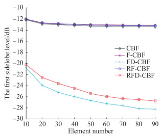Figure  4  First sidelobe level

Download: Full-Size Img

3.1.3   Root–mean–square error

For one target at 0°, the RMSE of DOA estimation is analyzed. The other parameters are kept constant.

Figure 5(a) shows that the RMSE curves decrease from 0.18 to 0 with the increase in the SNR from −21 dB to 15 dB. Figure 5(b) shows that the RMSE curves decrease from 0.032 to 0 with the increase in the SNR from 0 dB to 15 dB. Moreover, the RMSEs of the FD-CBF and RFD-CBF are lower than those of the F-CBF and RF-CBF, indicating that the focused-and-deconvolved method can well enhance the RMSE of DOA estimation.

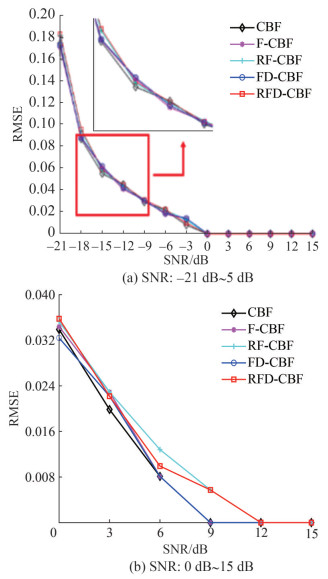Figure  5  Root–mean–square error (RMSE)

Download: Full-Size Img

3.2   DOA estimation

Two targets of equal strength (0 dB) are used to analyze the bearing resolution performance.

By changing the bearing interval of two targets, Figures 6(a) and 6(b) show that the bearing resolution of FD-CBF is 1.1°, and Figures 6(c) and 6(d) show that the bearing resolution of RFD-CBF is 1.2°. Therefore, we have proven that compared with CBF, the focused-and-deconvolved method can enhance the bearing resolution performance.

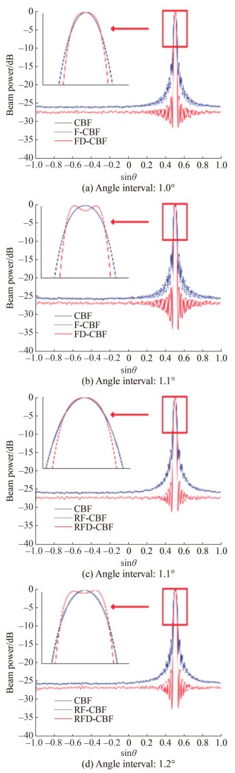Figure  6  Bearing resolution

Download: Full-Size Img

To further investigate the bearing resolution performance, Figure 7 shows the bearing time records (BTRs) of CBF, FD-CBF, and RFD-CBF. The dynamic target (1) moves from −35° to −30°, with an SNR of −5 dB. The static targets (2 and 3) are kept constant at 32° and 33.3°, with SNRs of 0 and −25 dB, respectively.

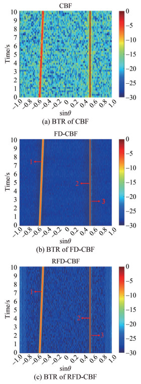Figure  7  Bearing-time records (BTRs)

Download: Full-Size Img

Figure 7(a) shows that a dynamic target (1) and a static target (2) exist in the BTR of CBF. By contrast, Figures 7(b) and 7(c) show that a weak target (3), which is obscured by the sidelobe level of the static target (2), can be detected. Therefore, the focused-and-deconvolved CBFs (FD-CBF and RFD-CBF) gets proved to suppress the sidelobe level and detect the weak target.

3.3   Anti-noise performance

Here, the average background level (ABL) (Sheng et al., 2020) and spatial spectrum gain (SSG) (Liu, 2021) are utilized to evaluate the anti-noise performance.

3.3.1   Average background level

Figures 8(a) and 8(b) show that the ABL decreases with the SNRs of [−30 dB, 15 dB] and [0 dB, 15 dB], respectively. Thus, we have proven that the ABL curves of CBF, F-CBF, and RF-CBF coincide and converge to −25 dB, whereas the ABL curves of FD-CBF and RFD-CBF are lower, reaching −38 and −40 dB, respectively. In summary, the focused-and-deconvolved method can suppress the ABL.

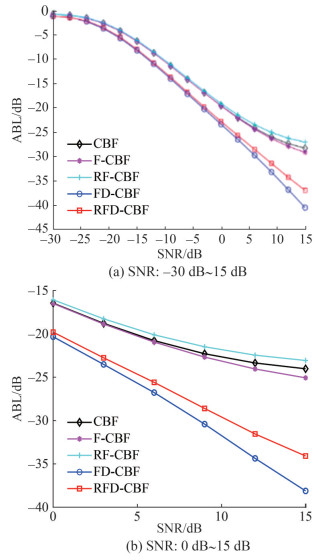Figure  8  Average background level (ABL)

Download: Full-Size Img

3.3.2   Spatial spectrum gain

The SSG is defined as follows:

where P(θ) and P_CBF(θ) are the spatial spectra of a certain beamformer and CBF, respectively, and θ ∈ (0, π) is the scanning angle.

Figures 9(a) and 9(b) show that the SSG increases with the SNRs of [−30 dB, 15 dB] and [0 dB, 15 dB]. The SSGs of F-CBF and RF-CBF are kept constant at 0 dB, indicating that the focusing transform does not affect the output SNR. The SSG curve of FD-CBF (RFD-CBF) increases from 0.5 dB to 3.2 dB (3 dB), indicating that deconvolution causes an increase in the output SNR. Thus, we have proven that the focused-and-deconvolved method can increase the output SNR, thereby enhancing the anti-noise performance.

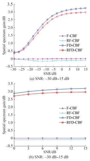Figure  9  Spatial spectrum gain (SSG)

Download: Full-Size Img

4   Data processing

A sea trial of underwater target detection was conducted in the South China Sea, approximately 100 km far from the coastline of Sanya City, on September 24 and 25, 2020.

The entire sea trial included a launching vessel with a transmitting sound source, a receiving vessel with a horizontal ULA, and a reserved noncooperative vessel. A low-frequency transducer (Model UW350) was selected as the transmitting sound source, with the source level set as 150 dB. A 128-element ULA operating at 120 Hz was used to collect data. Noncooperative targets, such as fishing boats, appear occasionally but do not affect the trial.

4.1   High bearing resolution performance

Figure 10 shows the BTRs of CBF, FD-CBF, and RFD-CBF processed using the sea trial data of 100 s.

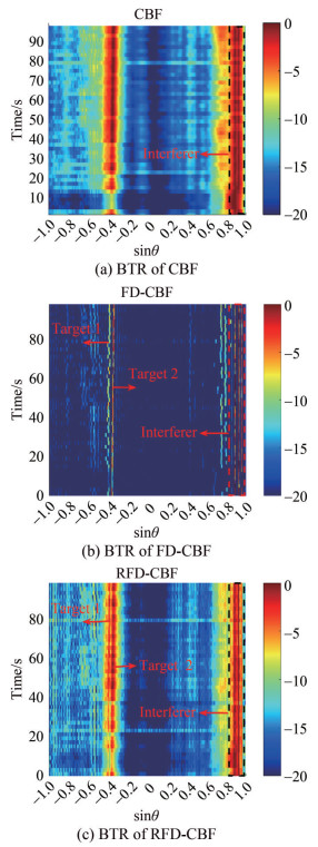Figure  10  Sea trial data processing Ⅰ

Download: Full-Size Img

Compared with Figure 10(a), Figure 10(b) shows that FD-CBF can spatially distinguish two neighboring targets, i. e., 1 and 2, with prior knowledge of target angles. By contrast, Figure 10(c) shows that RFD-CBF can spatially distinguish two adjacent targets, i.e., 1 and 2, without prior knowledge of target angles. However, a few false targets are detected in Figure 10(b), although their background levels are slightly lower than those detected in Figure 10(c).

Thus, we have proven that the focused-and-deconvolved method can enhance the bearing resolution performance and suppress the background level to some extent.

4.2   Weak target detection

Figure 11 shows the BTRs of CBF, FD-CBF, and RFD-CBF processed using the sea trial data of 100 s.

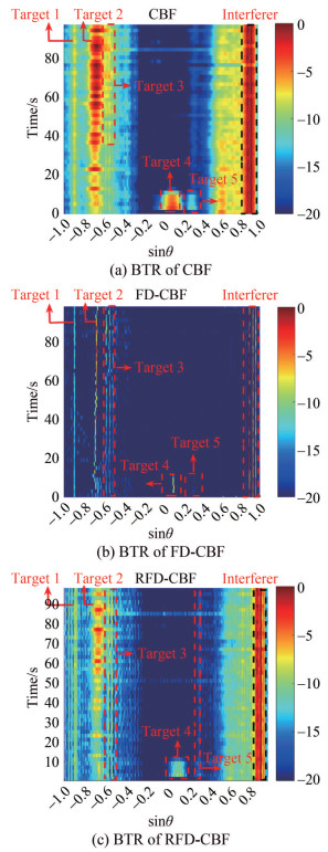Figure  11  Sea trial data processing Ⅱ

Download: Full-Size Img

Figure 11 shows two weak targets, i.e., 3 and 5, where the strength of Target 5 is slightly lower than that of Target 3. As shown in Figure 11(a), Target 3 appears from 40 to 100 s and disappears from 0 to 40 s, which can be attributed to the fact that the weak target (3) is obscured by the sidelobe level of the static target (2). Similarly, when the strength of Target 5 is low and even close to the background level, Target 5 appears from 0 to 10 s and disappears from 10 to 100 s. As shown in Figure 11(b), with prior knowledge of target angles, FD-CBF can detect the weak target (3) from 0 to 100 s, whereas the weak target (5) can be vaguely detected from 0 to 10 s. Compared with Figures 11(a) and 11(b), Figure 11(c) shows that RFD-CBF can detect Target 3 (Target 5) with a neighboring loud source, i. e., Target 2 (Target 4), from 0 to 100 s, without prior knowledge of target angles.

Thus, we have proven that RFD-CBF exhibits excellent performance in weak target detection.

5   Conclusion

In this paper, a focused-and-deconvolved method is proposed to address the wide mainlobe and high sidelobe levels of wideband CBF based on focusing transform and deconvolution. First, the focused-and-deconvolved beam power (FD-CBF and RFD-CBF) is simulated and evaluated in terms of the mainlobe width, first sidelobe level, and RMSE. Then, DOA estimation is analyzed in terms of the bearing resolution performance and BTRs. Subsequently, anti-noise performance is assessed from aspects of the ABL and SSG. Finally, considering the feasibility of practical application, RFD-CBF is confirmed to be more suitable for actual data processing without prior knowledge of target angles, compared with FD-CBF.