1   Introduction

The effectiveness of sonar in remotely detecting, locating, extracting, and recognizing target signals in underwater environments greatly depends on the signal processing technology employed by underwater acoustic arrays. Among these technologies, DOA estimation plays a pivotal role in the realm of underwater acoustic array signal processing. In recent decades, there has been a proliferation of super-resolution DOA estimation algorithms tailored for under-water detection. Notable examples include the multiple signal classification (MUSIC) method (Wagner et al., 2021) and the estimation of signal parameter via rotational invariance technique (ESPRIT) method (Li et al., 2020).

While subspace-based DOA estimation algorithms like MUSIC can achieve super-resolution DOA estimation, they are not without their limitations. For instance, these algorithms rely on eigenvalue decomposition of the data covariance matrix and the exhaustive search of all spatial angles, resulting in prohibitively high computational complexity (Guo et al., 2022). Furthermore, the majority of subspace-based DOA estimation algorithms exhibit limited adaptability when confronted with scenarios involving small snapshots, low SNR, and correlated signals. In contrast, sparse reconstruction-based DOA estimation algorithms excel in adapting to such challenging conditions.

In recent years, the application of sparse signal representation (Chen et al., 2001; Donoho et al., 2006) and compressed sensing (Donoho, 2006) has emerged as a powerful mathematical tool in the realm of DOA estimation. Notably, Malioutov et al. (2005) introduced a groundbreaking sparse representation model based on the l₁-norm penalty for DOA estimation, commonly known as the l₁-SVD method. This method entails performing singular value decomposition (SVD) on the data matrix to reduce its dimensionality and subsequently solving it through a second-order cone (SOC) program. In parallel, Stoica et al. (2011) proposed the sparse iterative covariance basis estimation (SPICE) method for DOA estimation, centered around the minimization of covariance matching criteria. These sparse reconstruction-based DOA estimation methods exhibit superior performance compared to traditional DOA estimation algorithms. However, a noteworthy limitation is their presumption that the DOAs of signals align precisely with predetermined angular grids, which is often overly idealistic. Consequently, these methods frequently encounter grid mismatch issues, leading to a reduction in DOA estimation accuracy.

In addressing the challenge of grid mismatch, researchers have introduced DOA estimation methods based on an off-grid model (Zhu et al., 2011; Gretsistas and Plumbley, 2012; Jagannath and Hari, 2013; Tan et al., 2014; Wu et al., 2018; Yang et al., 2013; Zhang et al., 2019). Zhu et al. (2011) employed the perturbation parameter method in DOA estimation, resulting in the development of a sparse total least squares method. Nevertheless, this method presents difficulties in parameter selection. Yang et al. (2013) leveraged first-order Taylor expansion to construct an offgrid model and introduced an off-grid sparse Bayesian inference (SBI) DOA estimation method. Tan et al. (2014) incorporated the structured error of the array manifold dictionary set into DOA estimation, proposing a model capable of jointly estimating sparse signals and grid offset errors. Zhang et al. (2019) adopted the iterative sparse projection (ISP) model (Sadeghi and Babaie-Zadeh, 2016) as a sparse signal recovery model, coupling it with the first-order Taylor expansion off-grid model to create a high-performance DOA estimation method. Recently, Dai et al. (2024) introduced a second-order Taylor expansion off-grid model, demonstrating enhanced DOA estimation accuracy under low SNR conditions when compared to the first-order Taylor expansion off-grid model.

With the evolution of sparse signal recovery theory, there is potential to devise more advanced DOA estimation methods that exhibit superior performance. The sparse signal representation model introduced by Sadeghi and Babaie-Zadeh (2016) lacks extrapolation steps and employs smoothing functions to address non-convex and non-smooth problems, leaving room for enhancing its sparse signal representation model. In this regard, Ghayem et al. (2018) adopted non-convex and non-smooth functions to portray the sparse signal model. They employed the IPP method to resolve the sparse signal representation model. The IPP method includes an extrapolation step, further augmenting its performance. Chen et al. (2020) applied the IPP method as a sparse signal representation model in the context of DOA estimation for monostatic Multiple-Input Multiple-Output (MIMO) radar, yielding commendable DOA estimation performance. However, it is worth noting that this method, as described, does not integrate with the off-grid model and consequently does not address grid mismatch issues.

In this study, we introduce the SCAD function as a non-smooth sparse promotion function into the sparse representation model for DOA estimation in underwater detection. The devised DOA estimation algorithm leverages the IPP method to solve the sparse representation model. Hence, the sparse signal recovery method employed in this study exhibits superior capability in recovering sparse signals, leading to a notable enhancement in DOA estimation accuracy compared to ISP method employed in Zhang et al. (2019). Subsequently, we propose a novel off-grid DOA estimation algorithm by combining the sparse representation model with an off-grid model constructed through first-order Taylor expansion. Simultaneously, the off-grid model, constructed through first-order Taylor expansion, effectively addresses the grid mismatch problem not accounted for in the framework proposed in Chen et al. (2020). This significantly contributes to the ultimate achievement of accurate DOA estimation.

2   Off-grid DOA estimation model

Assuming the presence of Q far-field narrowband signals, denoted as s_q(t) for q = 1, 2, …, Q from Q distinct directions (θ₁, θ₂, …, θ_Q), and incident upon a uniform linear array (ULA) consisting of M elements. In this ULA, the separation between adjacent elements is set to half the wavelength of the signal. The kth snapshot signal data vector received by the ULA can be expressed as:

where $\boldsymbol{x}(k)=\left[x_1(k), \cdots, x_M(k)\right]^{\mathrm{T}}$ represents the kth snapshot signal data vector received by ULA, $\boldsymbol{\theta}=\left[\theta_1, \theta_2, \cdots\right., \left.\theta_Q\right]^{\mathrm{T}}$, and n(k) signifies an independent identically distributed Gaussian white noise signal with a zero mean. $\boldsymbol{A}(\boldsymbol{\theta})=\left[\boldsymbol{a}\left(\theta_1\right), \cdots, \boldsymbol{a}\left(\theta_Q\right)\right]$ represents the array manifold matrix, where the qth steering vector of A(θ) is denoted as $\boldsymbol{a}\left(\theta_1\right)=\left[1, e^{-j {\rm{ \mathsf{ π} }} \sin \theta_q}, \cdots, e^{-j(M-1) {\rm{ \mathsf{ π} }} \sin \theta_q}\right]^{\mathrm{T}}$.

The spatial range of [−90°, 90°] is divided into a set of search angles $\overline{\boldsymbol{\theta}}=\left\{\bar{\theta}_1, \cdots, \bar{\theta}_G\right\}$ with equally spaced angular intervals denoted as ‘b’, where $G \gg Q$ signifies the number of grid points. In cases where the qth DOA of the signal does not precisely align with a grid point, that is, $\theta_q=\bar{\theta}_{g q}+\beta_q \notin \overline{\boldsymbol{\theta}}$ and $\bar{\theta}_{g q} \in \overline{\boldsymbol{\theta}}$, we employ first-order Taylor expansion to approximate the true steering vector of the qth signal. This approach enables us to:

where $\left|\beta_q\right| \leqslant \frac{b}{2}$ signifies the absolute value of the associated grid offset, with θ_gq representing the nearest grid point to the DOA.

Let’s define Φ as a diagonal matrix, denoted as Φ = diag(β), where $\boldsymbol{\beta}=\left[\beta_1, \cdots, \beta_G\right]^{\mathrm{T}}$. Furthermore, there is $\boldsymbol{B}(\overline{\boldsymbol{\theta}})=\left[\boldsymbol{a}^{\prime}\left(\bar{\theta}_1\right), \cdots, \boldsymbol{a}^{\prime}\left(\bar{\theta}_N\right)\right]$, and the resulting modified array manifold dictionary set matrix is then:

When the array receives data from K snapshots, the matrix representing the received data by the array can be expressed as:

where $\boldsymbol{X} \boldsymbol{\epsilon} \mathbb{C}^{M \times K}, \tilde{\boldsymbol{S}} \boldsymbol{\epsilon} \mathbb{C}^{N \times K}$ denotes the unknown sparse signal matrix, and $\boldsymbol{N} \boldsymbol{\epsilon} \mathbb{C}^{M \times K}$ is the noise data matrix.

Here, we define an indicator function:

and the mixed norm of $\|\tilde{\boldsymbol{S}}\|_{2, 0}$ is

It is evident that among all grid points, only Q grid points exhibit signal presence. As a result, $\tilde{\boldsymbol{S}}$ constitutes a row-sparse signal matrix, which can be reconstructed employing sparse signal recovery theory. In other words:

where ε represents the admissible noise threshold and ‖∙‖_F stands for the Frobenius norm. It is well-recognized that minimizing the l₀-norm poses an NP-hard problem. To address this challenge, various approaches have been employed, such as the use of smooth convex functions like the l₁-norm or non-convex smoothing functions like the l_p-norm to approximate it (Elad 2010). However, employing convex or smooth functions to represent non-convex and non-smooth sparse signal recovery problems can introduce model inaccuracies. Fortunately, recent advances in sparse signal recovery have indicated that the selection of appropriate non-convex and non-smooth sparse promotion functions can yield superior sparse recovery results compared to other relaxation techniques (Ghayem et al., 2018).

3   Proposed off-grid DOA estimation method for passive sonar detection based on IPP

In this section, we will employ the concept of alternating optimization iterations in conjunction with the IPP method to solve equation (7). Prior to commencing the i + 1th iteration, we have acquired (or set) the values of $\tilde{\boldsymbol{S}}_i$ and β_i. Subsequently, we can determine the values of $\tilde{\boldsymbol{S}}_{i+1}$ and β_{i + 1} for the i + 1th iteration through the following process:

and

3.1   Restore the unknown sparse signal matrix

To attain the sparse solution as indicated in equation (8), the DOA estimation problem in passive sonar can be reformulated into an optimization problem involving the proximal function (Parikh and Boyd, 2014). This transformation yields:

where H(Z) represents a non-convex and non-smooth sparse promotion function, while Γ_Αε denotes the indicator function (Eftekhari et al., 2009) of set $\mathrm{A}_{\varepsilon} \triangleq\left\{\overline{\boldsymbol{S}}_i:\right.\left.\left\|\boldsymbol{X}-\left[\boldsymbol{A}(\overline{\boldsymbol{\theta}})+\boldsymbol{B}(\overline{\boldsymbol{\theta}}) \boldsymbol{\varPhi}_i\right] \overline{\boldsymbol{S}}_i\right\|_{\boldsymbol{F}}^2 \leqslant \varepsilon\right\}$. This leads to:

By incorporating the norm penalty method (Nocedal and Wright, 1999) into the sparse signal representation model presented in equation (10), we have

in which υ > 0 denotes a penalty parameter. The alternating minimization method can solve (12), there is

In line with the proximal projection definition (Parikh and Boyd, 2014), equation (13) can be streamlined to:

where $\operatorname{prox}_{v H}\left(\overline{\boldsymbol{S}}_i\right)$ represents the proximal operator of υH(Z). Furthermore, the inclusion of an extrapolation step (Nesterov, 2004) significantly enhances the performance of the IPP algorithm, resulting in:

in which a ≥ 0 denotes a weighting constant. To express equation (14) in a more concise and compact form, we have:

where P_Αε represents the projection of set Α_ε.

In a study by Ghayem et al. (2018), it was showcased that the fusion of the SCAD function (Fan and Li, 2001) as a sparse promotion function with IPP methods outperforms other non-smooth functions in terms of performance. For computational convenience, we employ $\overline{\boldsymbol{S}}_i^{l 2}$ to denote the column vector formed by the l₂-norm of each row vector in matrix $\overline{\boldsymbol{S}}_i$. Consequently, we have:

in which the $\boldsymbol{F}_{\tau, w}^{\mathrm{scad}}\left(\overline{\boldsymbol{S}}_i^{l 2}\right)$ represents the proximal mapping of SCAD function. And there is

in which w > 2, τ > 0 represents a threshold constant and $(s)_{+} \triangleq \max (s, 0)$. Upon obtaining the sparse vector through the solution of equation (16), the DOAs of the target can be determined by locating the position of the spectral peak.

Considering that the primary emphasis of this article lies in the application of the IPP algorithm to devise DOA estimation methods with robust sparse signal recovery capabilities, and given that prior mathematical studies (Ghayem et al., 2018) have extensively detailed the utilization of the SCAD function and proximal operator for sparse signal recovery within the IPP algorithm, this paper places greater focus on the conclusive nature of employing the SCAD function and proximal operator.

3.2   Update grid offset β

In order to obtain the grid offset parameter β_{i + 1} after acquiring the sparse signal matrix $\overline{\boldsymbol{S}}_{i+1}$, we solve equation (9). This can be expressed as follows:

in which A₁ denotes A(θ), B₁ represents B(θ). Let’s define

and (19) is equivalent to:

In (21), Π(β_i) represents a convex function. In accordance with the principles of convex optimization theory, for a continuously quadratic differentiable and convex function Π(β_i), its minimum value is attained when

where Δ(∙) denotes derivative symbol. And easy to obtain

in which Re(.) represents the operator for extracting the real part, with the symbol○indicating the Hadamard product.

Table 1 presents a summary of the proposed off-grid DOA estimation method based on IPP. The key parameters outlined in Table 1 are as follows: a = 0.9, w = 30, I = 3, K = 0.9, $\tau_0=5 \cdot \max \left|\tilde{\boldsymbol{S}}_0(:, l)\right|$, in which $\left|\tilde{\boldsymbol{S}}_0(:, l)\right|$ denotes the modulus vector comprising all elements in the lth column vector of the matrix $\tilde{\boldsymbol{S}}_0$. It is crucial to note, as indicated in Table 2, the presence of an inner loop between the ith iteration and the i + 1th iteration. The steps involved in this inner loop are outlined in Table 1.

4   Analysis of simulation results

In this section, a significant number of simulation experiments were conducted to assess the performance of the proposed DOA estimation algorithm and to compare it with several state-of-the-art algorithms, including l₁-SVD (Malioutov et al., 2005), OGSBI (Yang et al., 2013), OG-ISP (Zhang et al., 2019), and IPP method (Chen et al., 2020). For all simulation experiments, an ULA with M = 18 sensors was employed to receive target signals. Unless otherwise specified, the number of signal snapshots in each simulation experiment was fixed at T = 100. Additionally, we considered Q = 2 uncorrelated far-field narrowband signals incident onto the ULA from angles of −10.3°and 10.3°, respectively. For all the simulation experiments, we maintained a grid spacing of b = 1° and conducted a total of MC=200 Monte Carlo operations. To quantitatively assess the DOA estimation accuracy of various algorithms, the root mean square error (RMSE) was employed as a performance metric, which is

where MC represents the number of Monte Carlo operations, θ^(p) represents the estimated DOAs, and θ^(p) represents the true DOAs in the pth experiment, respectively.

In Simulation 1, Figure 1 displays the normalized spatial spectrum of l₁-SVD, OGSBI, OG-ISP and the proposed OG-IPP methods. For this simulation, we considered Q = 2 uncorrelated far-field narrowband signals incident onto an ULA from angles of − 6.5°and 6.5°, respectively. The grid spacing was set to b = 1°, and the orientation of the target signal deviated by 0.5° from the nearest grid point. As illustrated in Figure 1, the l₁-SVD method exhibited the poorest performance due to its lack of integration with the off-grid model, resulting in a deviation of 0.5° from the true signal direction. In comparison, the OGSBI method showed improved performance, with an estimated target signal orientation deviating by 0.1° from the true orientation. Furthermore, both the proposed method and OG-ISP accurately estimated the target orientation, aligning perfectly with the true orientation of the target signal, thereby demonstrating excellent DOA estimation performance.

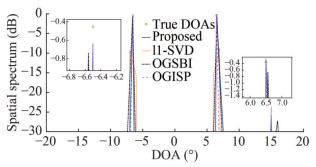Figure  1  Normalized spatial spectral performance of different algorithms (SNR=0 dB)

Download: Full-Size Img

In Simulation 2, the RMSE performance of l₁-SVD, OGSBI, OGISP and the proposed OG-IPP methods under various input SNR is depicted in Figure 2 through Figure 5. In Figures 2 and 3, the number of snapshots for each algorithm was set to T=50, with corresponding array elements of M=18 and M=20, respectively. From the observations made in Figure 2 and Figure 3, it is evident that the l₁-SVD algorithm inherently suffers from grid bias, leading to an inability to enhance DOA estimation accuracy as SNR increases. Conversely, off-grid DOA estimation methods can overcome grid mismatch issues, with RMSE approaching 0 as SNR continues to rise. Notably, among the three offgrid DOA estimation methods, the proposed method exhibits the lowest RMSE, indicating the highest DOA estimation accuracy. In Figures 4 and 5, each algorithm was provided with T=100 snapshots, and the corresponding number of array elements was M=18 and M=20, respectively. Similar to Figures 2 and 3, the proposed method consistently demonstrated the lowest RMSE among the three off-grid DOA estimation methods in Figure 4 and Figure 5. Across these four distinct conditions, involving varying input SNR, snapshot number, and array element number, it can be concluded that the proposed method consistently exhibits the lowest RMSE curve, signifying superior DOA estimation accuracy.

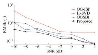Figure  2  The RMSE performance versus SNR (T=50, M=18)

Download: Full-Size Img

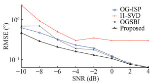Figure  3  The RMSE performance versus SNR (T=50, M=20)

Download: Full-Size Img

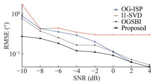Figure  4  The RMSE performance versus SNR (T=100, M=18)

Download: Full-Size Img

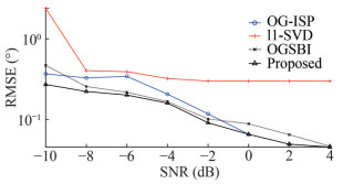Figure  5  The RMSE performance versus SNR (T=100, M=20)

Download: Full-Size Img

In Simulation 3, Figure 6 illustrates the RMSE performance of the proposed method as a function of SNR with different numbers of array elements. For Simulation 3, the number of snapshots was set to T=50. As evident from Figure 6, an increase in the number of array elements results in a gradual improvement in the DOA estimation accuracy of the proposed method. In essence, the greater the number of hydrophone arrays, the larger the array aperture that can be formed, leading to improved spatial resolution and, consequently, enhanced DOA estimation performance. This phenomenon can be attributed to the benefits of waveform diversity gain.

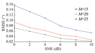Figure  6  The RMSE performance of proposed method versus number of array elements

Download: Full-Size Img

In Simulation 4, the RMSE performance of IPP DOA estimation method (Chen et al., 2020) and the proposed OG-IPP method under various input SNR is depicted in Figure 7. From Figure 7, it is evident that as the SNR increases, the accuracy of DOA estimation improves for both algorithms. Nonetheless, because the IPP method did not incorporate an off-grid model, the RMSE of DOA estimation remained constant even as the input SNR exceeded −8dB. In contrast, the proposed OG-IPP method, which integrates off-grid models, demonstrates a reduced RMSE and the capability to mitigate grid mismatch issues. With a continued increase in the input SNR, the RMSE of DOA estimation gradually converges towards 0.

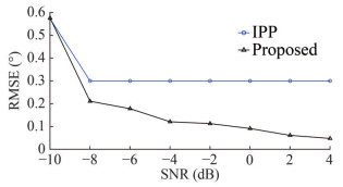Figure  7  The RMSE performance versus SNR (T =100, M =20)

Download: Full-Size Img

5   Data processing

To validate the algorithm’s effectiveness, underwater target detection experiments were conducted in the South China Sea in September 2020. A fiber optic hydrophone array system, featuring an ULA comprising twenty sensors, was deployed on the seabed. The ULA has an array element spacing of 6.25 meters and was positioned at a depth of approximately 120 meters within the designated sea area. The observation range of the ULA extended from [−90°, 90°]. According to GPS navigation data, the ship receiving the sound source is positioned at the azimuth of 65° relative to the array. Additionally, another type of experimental cooperative target ship is located around the azimuth of 50° relative to the array.

In this underwater target detection experiment, the processed data spanned a duration of 400 s, which was divided into 20 segments, each lasting 20 s. The dataset used in the experiment was gathered between 13:23 and 13:29 on September 24, 2020, during the midday hours. Throughout the data processing in the sea trial, a far-field narrowband signal model was employed to both describe and process the data. In the course of the experiment, the cooperative target ship at 50° transmitted a single-frequency signal with a signal frequency of 73 Hz. Consequently, the narrowband signal frequency chosen for processing was set to 73 Hz. The array receiving data was sampled at a rate of 32 000 Hz, necessitating FFT transformations every 32 000 data points. For DOA estimation purposes, the algorithm generated spatial spectra plots every 20 snapshots in the frequency domain and produced Bearing-Time Records (BTRs) every 2 s.

During the processing of the sea trial data, four DOA estimation methods—CBF, OGSBI, OG-ISP, and OG-IPP—were employed to analyze and determine the DOAs of targets within the sea trial area. Figure 8 presents the results of CBF processing on the sea trial data. It is evident that the main lobe of the CBF spatial spectrum is excessively broad, allowing only a rough determination of the target’s azimuth range. This limitation makes it challenging to precisely measure the direction of the target. Hence, the CBF algorithm is unable to differentiate between cooperative targets at 50° and ship targets receiving sound sources at 65°. Furthermore, the CBF algorithm detected a non-cooperative target in the vicinity of the −20 degrees orientation. Figures 9 to 11 display the BTRs generated by the OGSBI, OG-ISP, and OG-IPP algorithms, respectively. From Figures 9 to 11, it becomes apparent that all three algorithms accurately detected the strong interference targets at − 20° and the sound source receiving ship targets at 65°. Moreover, they also successfully detected a weaker target at 50°, a task for which the CBF algorithm demonstrated subpar azimuth estimation accuracy, failing to detect any target at 50°. Furthermore, it is worth noting that the proposed algorithm’s target tracking trajectory appears the narrowest among the three algorithms, indicating the highest DOA estimation performance among them.

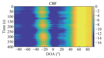Figure  8  BTRs of CBF

Download: Full-Size Img

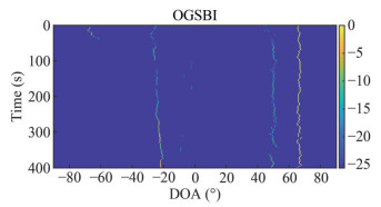Figure  9  BTRs of OGSBI

Download: Full-Size Img

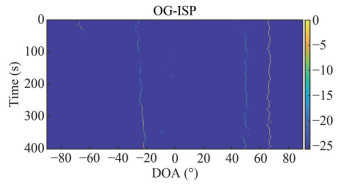Figure  10  BTRs of OG-ISP

Download: Full-Size Img

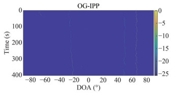Figure  11  BTRs of OG-IPP

Download: Full-Size Img

6   Conclusions

This paper introduces a novel high-performance off-grid DOA estimation method based on IPP. In the proposed method, an alternating optimization strategy is utilized to jointly estimate sparse signals and grid offset parameters. We employ a proximal function optimization model to address the non-convex and non-smooth sparse representation challenges in DOA estimation. Additionally, the SCAD function is employed to derive the proximal operator for solving the model. As a result, the proposed algorithm exhibits robust sparse signal recovery capabilities and delivers more accurate DOA estimation results. Through simulations and sea trial experiments, the proposed approach has demonstrated superior resolution and more precise DOA estimation performance in comparison to traditional sparse classification methods and advanced off-grid methods. While the proposed algorithm demonstrates high accuracy in DOA estimation, it comes with a high computational complexity. There remains a gap in achieving real-time processing for seamless integration into the detection system. Additionally, there is potential for improvement in the first-order Taylor expansion off-grid model. A future direction could involve exploring the use of multi-order Taylor expansion terms to design off-grid models, aiming to further enhance the accuracy of DOA estimation.