1   Introduction

Synthetic fiber ropes have attracted attention in industries, and polyester has become a popular mooring material due to its lightweightness, low cost, corrosion resistance, and high strength (Flory et al., 2007; Lian and Liu, 2019). However, polyester exhibits inconsistent axial stiffness characteristics, and load history affects rope performance (Banfield et al., 2010). Given this complex nonlinear behavior, the development of models that represent precisely the stiffness characteristics of rope presents difficulty (Kim et al., 2003). In general, this phenomenon is described using dynamic stiffness, which refers to the ratio of the difference between the peak and valley of tension and the corresponding elongation of synthetic fiber rope under cyclic load (Davies et al., 2002).

Studies have been conducted on dynamic stiffness. The work of Vecchio (1992) on dynamic stiffness led to the proposal of an empirical expression that explains the effects of mean tension, tension amplitude, and load period on the dynamic stiffness of rope and the promotion of engineering applications of synthetic fiber rope in deepwater mooring. François and Davies (2008) conducted an experimental study on the dynamic stiffness of polyester, aramid, and high-modulus polyethylene cables and proposed an empirical expression that describes the influence of the mean tension of cables on dynamic stiffness. Liu et al. (2014) performed cyclic load tests on polyester, aramid, and high-modulus polyethylene cables and proposed an expression considering the effects of mean tension, strain amplitude, and load cycles of cables. In order to gain insights into the dynamic stiffness of synthetic fiber ropes, many researchers (Casey and Banfield, 2002; Wibner et al., 2003; Tahar and Kim, 2008) have proposed the use of various empirical expressions for dynamic stiffness. Although the expressions vary with different rope samples, they reflect the effect of mean load on dynamic stiffness.

However, the expressions mostly come from cyclic tests (Li et al., 2021; Chang et al., 2012) and are difficult to apply in actual sea conditions as irregular waves lack an evident periodicity. Consequently, the effects of load amplitude, loading period, and load history have been explored to discuss the deformation of expressions for improved applications in random seas (ABS, 2011). Currently, the ABS (2011) (American Bureau of Shipping) and DNV (2015) (Det Norske Veritas) standards have provided empirical practices, and most commercial software can handle the dynamic stiffness model. However, the values of the model are often arbitrarily determined by users, which may lead to distorted simulation results (Mao, 2019).

In this paper, an innovative method for the calculation of the dynamic behavior of polyester rope was proposed based on the dynamic stiffness model. In addition, a related simulation program that fixes the arbitrary issue due to human factors because the values of the dynamic stiffness model are determined by the program automatically was developed.

2   Theoretical method

2.1   Equation for dynamic stiffness

Fiber rope stiffness is expressed as follows:

where ΔF refers to the change in load, Δε denotes the change in strain, and EA indicates the stiffness or modulus times the cross-sectional area of the rope. Equivalently, a nondimensional stiffness K_r can be expressed as follows:

where MBS represents the minimum breaking strength.

The three-parameter equation is recommended fordynamic stiffness K_rd (ABS, 2011):

where L_m is the mean load of MBS in %, T is the load amplitude of MBS in %, P is the loading period, and α, β, γ and δ represent the coefficients related to the physical characteristics of fiber rope (Liu et al., 2014).

Based on the studies of Vecchio (1992), Casey and Banfield (2002), and Depalo et al. (2022), this paper removes the tension amplitude and loading period from the equations, which implies that the mean load remains the key parameter in the simulation of polyester rope in nonlinear environments.

Consequently, Equation (3) can be simplified as follows:

The coefficients in Equation (4) can be obtained through cyclic load tests. Moreover, related works have been conducted, and empirical expressions have been proposed (François and Davies, 2008; Casey and Banfield, 2002; Wibner et al., 2003).

In this paper, the dynamic stiffness model was referred to the work of Davies (François and Davies, 2008), and the detailed expression of Equation (4) was computed as follows:

2.2   Analysis procedure

The mean load L_m is hard to determine in a random sea. The current standard, DNV (2015), proposes a practical mooring analysis procedure that considers the effect of dynamic stiffness of synthetic fiber ropes; the procedure can be summarized as follows:

1) Perform static analysis using appropriate nonlinear working curves that consider mean environmental loads.

2) Determine the mean tension (L_m) at the fairlead, calculate dynamic stiffness using L_m (equation (5)), and update the model using the axial stiffness value.

3) Perform static and dynamic analyses using the updated mooring line properties.

This paper proposes a relatively complex calculation method. Compared with the DNV procedure, the most helpful function of this method is confirming the mean load L_m in Equation (5) automatically, which means that it can avoid meticulous iterations to find a proper value of L_m. Thus, this method may prevent distorted calculation results. Figure 1 shows the flow chart of the method.

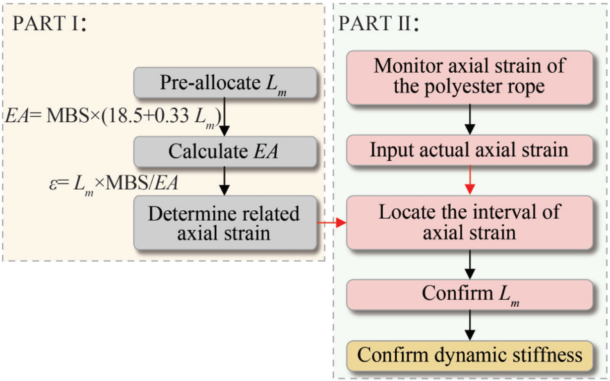Figure  1  Flow chart of the analytical procedure

Download: Full-Size Img

Part Ⅰ: This part mainly preallocates the mean tension L_m for calculation.

1) As L_m is a percentage of MBS, use 100 values for calculation. In other words, use the value of L_m every 1% for calculation. Moreover, implement the linear interpolation method to supplement every 1% interval.

2) Obtain the axial stiffness EA = MBS × (18.5 + 0.33 L_m) for the preallocated L_m.

3) Determine the axial strain ε = L_m × MBS/EA related to the EA in Step 2.

Part Ⅱ: This part determines the values of the mean tension L_m through real-time monitoring of the axial strain to confirm the dynamic stiffness.

1) Given the displacement of floating structures, monitor in real time the axial strain of each mooring line element and its changes over time.

2) Use the axial strain obtained in Step 1 as input and compare it with the strain in PART Ⅰ until both parameters reach equality.

3) Locate the actual axial strain interval.

4) Reverse all steps in PART Ⅰ and confirm the mean tension L_m.

5) Calculate the dynamic stiffness in Equation (5).

As indicated in the procedure, the analysis method is divided into two parts. The mean tension L_mrefers to the real-time environmental load. Consequently, some conditions may result in intense or mild simulation.

2.3   Absolute nodal coordinate formulation (ANCF)

Based on the analysis procedure, a simulation program in which the theoretical background originates from the ANCF was developed (Shabana and Yakoub, 2001). Given its strong nonlinearity, including large axial deformation, the polyester rope cannot be simulated precisely due to the low strain assumption. However, ANCF is not limited by such an assumption and thus can handle the mentioned issue (Li et al., 2022).

ANCF defines nodal element coordinates, including the global displacement and slopes, in a fixed inertial coordinate system (Shabana (1997); Berzeri et al. (2001)). Hence, no transformation matrices are required to define the kinematic position and velocity equations of elements (Li et al., 2022). Motion equation can be defined as follows:

where M represents the mass matrix, q denotes the nodal coordinate, and Q_s and Q_e are the elastic and externally applied forces, respectively.

In ANCF, the nodal coordinate q of an element is defined in twelve terms (Gerstmayr and Shabana, 2006):

where q₁, q₂, and q₃ are the displacement terms, and q₄, q₅, and q₆ are the slope terms of the left node, which means that the other terms are parameters of the right node.

Elastic force Q_s can be defined using the strain energy U (Zhang et al., 2016):

where L refers to the total length of the structure, I corresponds to the area moment of inertia, and K_κ is the material point curvature.

Usually, the bending curvature term Q_s2 is disregarded in the calculation of mooring lines because of its large slenderness ratio, and the axial strain term Q_s1 is applied in the simulation (Zhang et al., 2019). Notably, with the change in axial stiffness EA, the elastic force changes nonlinearly.

The externally applied force Q_e is defined as follows:

where r = Sq represents the global position vector, and S corresponds to the shape function.

f refers to external forces, such as gravity, buoyancy, and wave forces, and the wave forces acting on a microelement ds can be obtained using the Morison equation (Kim et al., 2005):

where C_d and C_m denote the drag coefficient and added mass coefficient. D indicates the diameter of the mooring line, and v_s and $\dot{\boldsymbol{v}}_s$ refer to the velocity and acceleration of wave particles, respectively. $\dot{\boldsymbol{r}}$ and $\ddot{\boldsymbol{r}}$ correspond to the velocity and acceleration of the mooring line, respectively. A_m stands for the circular area of the mooring line. N is a 3D normal transformation matrix that ensures the perpendicularity of weave force direction to the mooring line:

3   Description of the numerical model

3.1   Pricipal dimensions

A deep draft semisubmersible platform is selected for calculation, and the hull dimensions are tabulated in Table 1.

Based on the main scale parameters listed in Table 1, the numerical model of the platform is established in SESAM software (Figure 2), and the hydrodynamic performance is obtained based on the potential flow theory.

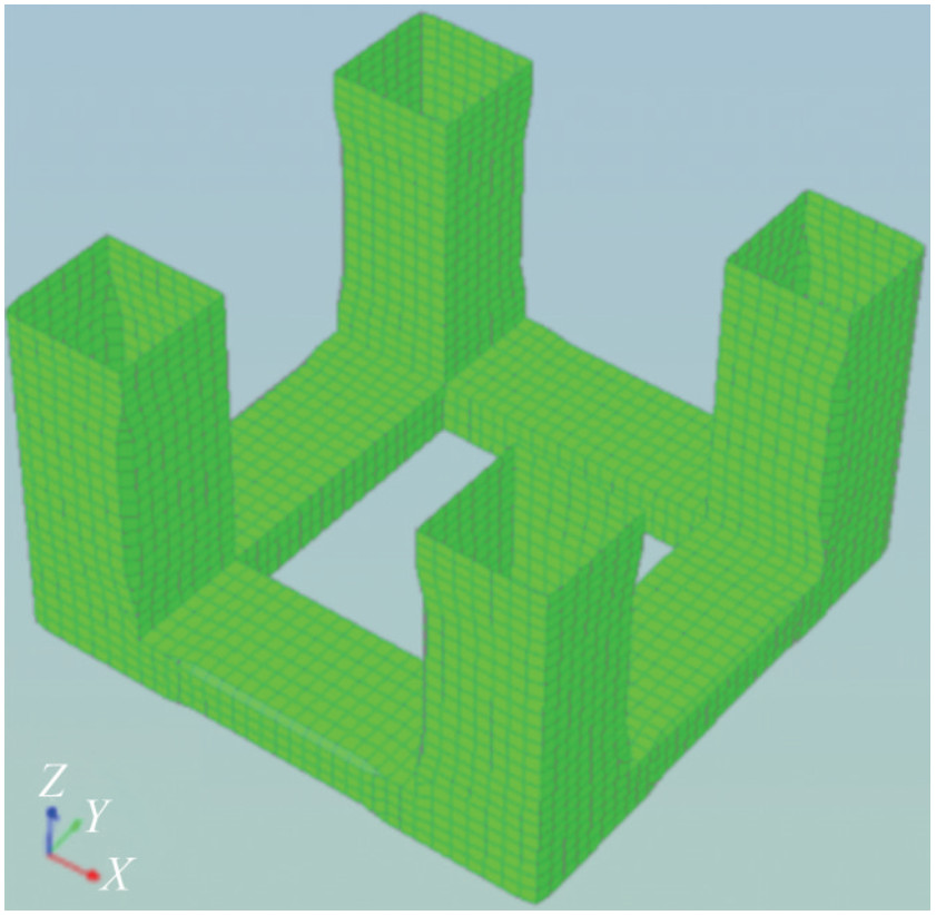Figure  2  Panel model of the semisubmersible platform in SESAM (HydroD)

Download: Full-Size Img

The hydrodynamic calculation results can be imported into the simulation program developed in this paper to conduct time-domain calculations. In addition, Orcaflex can use the results of SESAM to avoid errors from the frequency domain.

On this basis, the dynamic response of the platform is calculated using the program and Orcaflex following the DNV procedure for simple validation. Then, the program with the designed analysis method is used to simulate the same conditions.

3.2   Mooring system arrangement

A chain-polyester rope-chain mooring system consisting of the same four lines moors the semisubmersible platform. Table 2 presents the properties of the mooring line's main components.

Figure 3 shows a snapshot of the mooring system layout. Figure 4 displays the detailed component of a single mooring line. The same settings are applied in Orcaflex, as stated in Section 3.1.

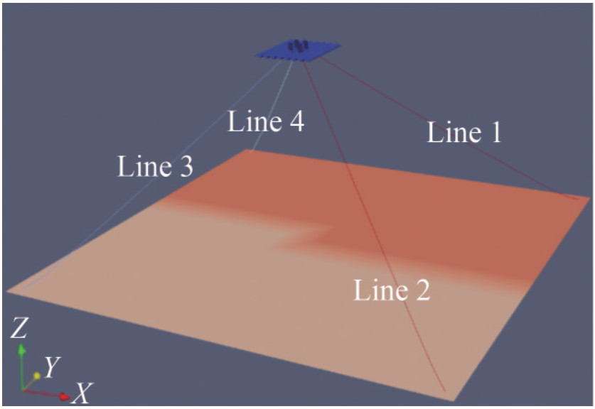Figure  3  Mooring arrangement of the semisubmersible platform

Download: Full-Size Img

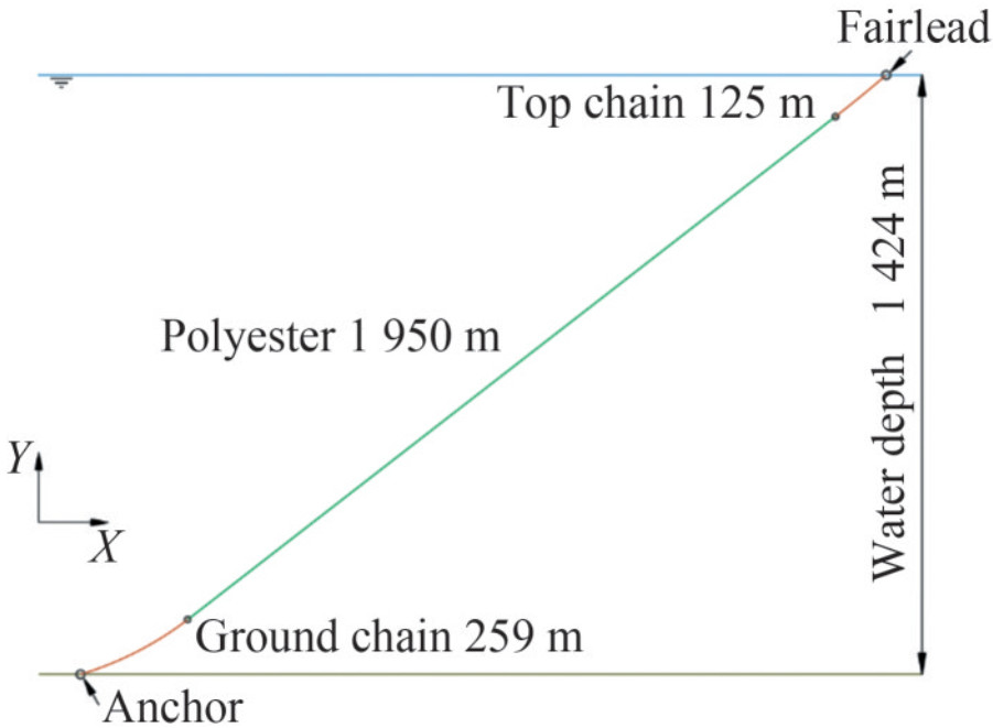Figure  4  Detailed diagram of a single mooring line

Download: Full-Size Img

3.3   Marine conditions

The semisubmersible platform serves in the South China Sea, with a water depth of approximately 1 200 m to 1 500 m. In this paper, the water depth is set to 1 424 m. Moreover, to gain further insights into the wave loads acting on the platform and mooring system, we exclude the simulation of wind and current loads in the calculation.

The Jonswap wave spectrum is applied in the calculation, and 1-, 10-, and 100-year return period conditions are considered as shown in Table 3. In addition, the wave direction of all three working conditions is set to 180°.

According to the data above, time-domain simulation is conducted using Orcaflex and the program developed in this paper.

4   Results and discussion

4.1   Motions of the semisubmersible platform

As the working conditions mainly include the heading wave, only the surge, heave, and pitch motions of the semisubmersible platform are analyzed because they are representative.

Figure 5 presents the statistical results for surge motion. Orcaflex provides the blue bar results. In addition, the yellow bar graph, which is also named MeanEA, is calculated using the program for comparison with Orcaflex. The program is also used to simulate the green bar results considering the real-time dynamic stiffness.

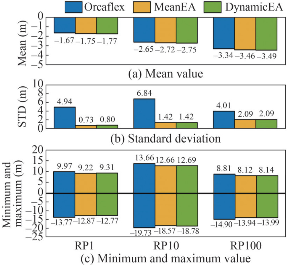Figure  5  Statistical results for surge motion

Download: Full-Size Img

Figure 5 shows the less discrepancy observed in the statistical results for surge motion. First, comparing the results of Orcaflex and MeanEA, the program can achieve a reliable simulation level. The errors are mostly within 10%. The results on MeanEA and DynamicEA show that the method proposed in this paper agrees well with the DNV procedure. However, the proposed method experiences a relatively inconvenient iteration in Step 2 of the DNV procedure. Thus, the results can achieve a good agreement. In addition, the standard deviation shows that the surge motion simulated by the program is relatively calmer than that produced by Orcaflex.

The mean offset of the platform increases with the severity of marine conditions. However, based on the maximum and minimum values, the most intense response of the platform appears in the 10-year return period scenario. Such a finding is observed mainly because the natural period of surge motion is almost the same as that of the wave spectrum. As a result, the motion response is magnified due to resonance.

An excellent agreement is also noticed in the heave motion of the semisubmersible platform shown in Figure 6. The statistical values show no noticeable changes in different working conditions. In addition, the maximum and minimum values increase as the environmental conditions aggregate.

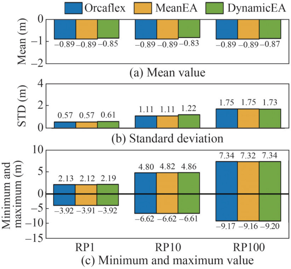Figure  6  Statistical results on heave motion

Download: Full-Size Img

Figure 7 displays the statistical results for the pitch motion of the semisubmersible platform. Similar to those of heave motion, the mean values of pitch motion are almost the same, and the maximum and minimum values are increased. In addition, the standard deviation presents minimal discrepancy, which means that the amplitude is the same around the mean value.

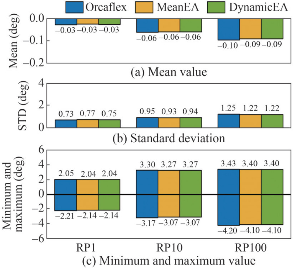Figure  7  Statistical results for pitch motion

Download: Full-Size Img

In general, given the motion responses in this section, the results on surge, heave, and pitch motions agree well with those of different calculation methods. The findings of Orcaflex and MeanEA indicate the ideal precision of the program developed in this paper and the reliability of the calculation method for dynamic stiffness. Moreover, the standard deviation of surge motion shows a discrepancy between Orcaflex and the program, and the heave and pitch motions show no notable error.

4.2   Axial tension of the mooring line

Differences between the two simulation procedures are reflected directly by the axial tension of the mooring lines. This section analyzes the statistical results for the four mooring lines. From the mooring layout in Figure 3, the tension response of Lines 1 and 2 present similar results to some degree because they are symmetrical along the X-axis. Lines 3 and 4 should present the same laws.

As shown in Figure 8, the mean tension between Orcaflex and MeanEA attains a maximum error of 4.68% under the 100-year return period condition. However, this error decreases to 0.04% under the same marine condition. Such finding is mainly due to the different calculation theories used by the two simulation tools (Li et al., 2022). The higher standard deviation of surge motion given by Orcaflex than that of the program leads to a similar condition of the standard deviation of the mooring lines.

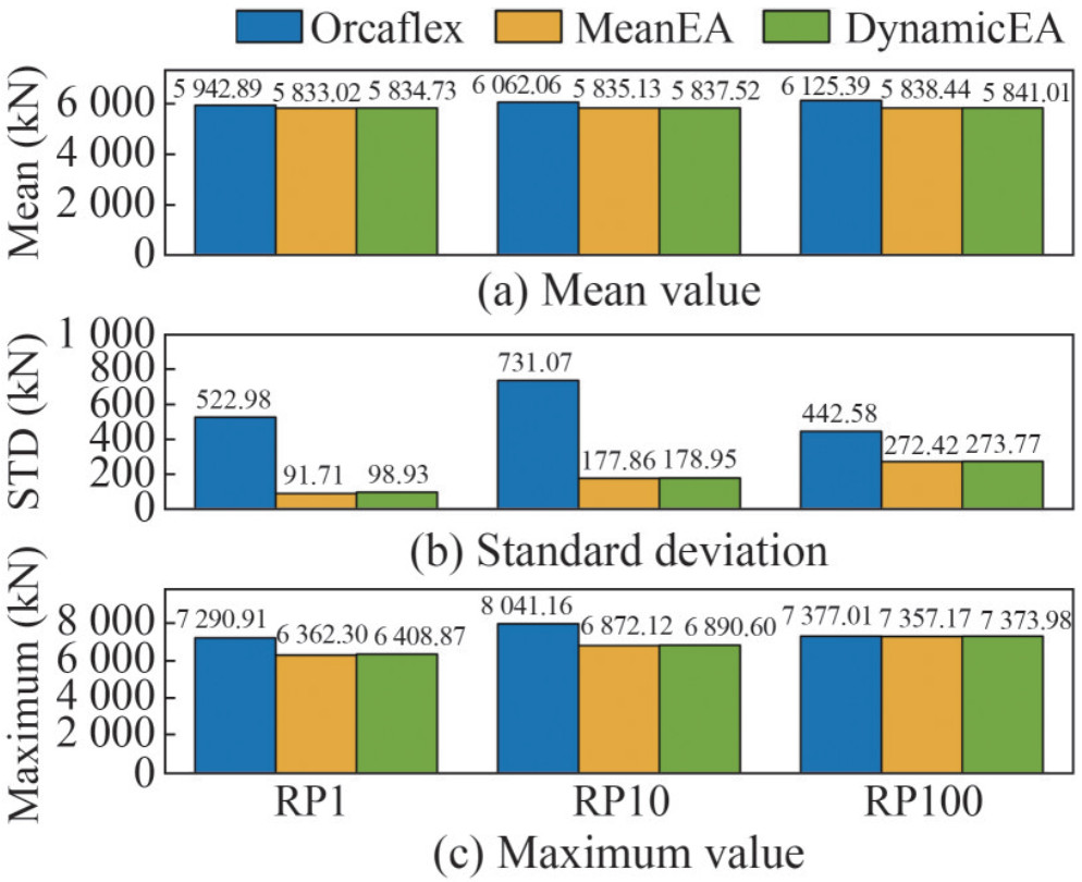Figure  8  Statistical results for the axial tension of mooring line 1

Download: Full-Size Img

The maximum tension of the mooring line occurs in the 10-year return period condition, and it is due to the resonance in the natural period of surge in the wave spectrum. In addition, the same conclusions are drawn for the other mooring lines.

The axial tension response of mooring line 2 shows the same phenomenon as line 1 in Figure 9, and the statistical values are almost similar to those of mooring line 1 due to symmetry.

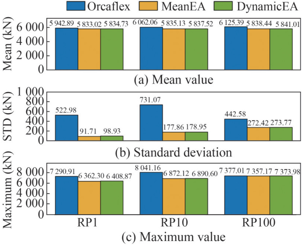Figure  9  Statistical results for the axial tension of mooring line 2

Download: Full-Size Img

Figure 10 shows the statistical results for the axial tension of mooring line 3. The mean tension between Orcaflex and MeanEA has a maximum error of 8.62% under the 100-year return period condition, and the errors between MeanEA and DynamicEA decrease to a low range. Given the resonance under the 10-year condition, the maximum tension of the mooring line is still larger than the other working conditions, which means the intense motion response of the semisubmersible platform.

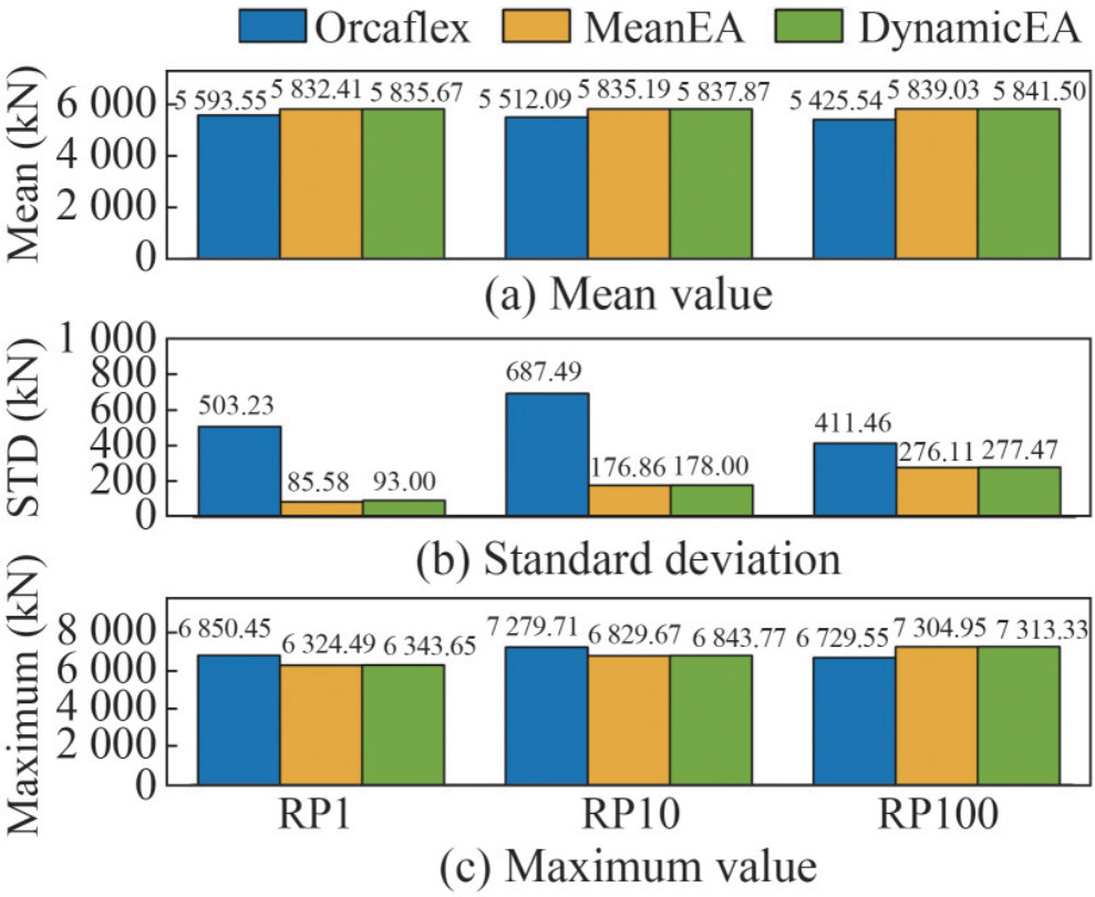Figure  10  Statistical results for the axial tension of mooring line 3

Download: Full-Size Img

In addition, the statistical results for the axial tension of mooring line 4 (Figure 11) are mostly the same as those of mooring line 3.

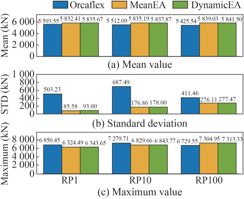Figure  11  Statistical results for the axial tension of mooring line 4

Download: Full-Size Img

The tension results of the mooring system relatively reach a good agreement through the two simulation procedures. The findings indicate the reliability of the method proposed in this paper for the calculation of the dynamic behavior of the polyester mooring system. However, the difference between the DNV procedure and the method proposed in this paper is determined using the mean load L_m. The former requires meticulous iteration, and a convenient practice is considering a dynamic stiffness equal to the multiple values of MBS (ABS, 2011), which leads to unreliable simulation findings. The method proposed can find the values of L_m automatically, as stated in the flow chart in Figure 1, and may avoid distorted calculation results.

5   Conclusions

In this paper, a newly designed calculation method is proposed to determine the dynamic stiffness of polyester rope. In the proposed method, monitoring of the axial strain of the rope shows real-time changes in the values. First, the results of Orcaflex and the program are compared following the DNV procedure to validate the reliability of the developed program. Then, the MeanEA and DynamicEA results are compared to determine the differences between the two simulation procedures. The main conclusions are drawn as follows:

1) Comparison of Orcaflex and the proposed program shows the reasonable calculation capability of the latter.

2) The method proposed in this paper for determining dynamic stiffness can conveniently reflect the dynamic behavior of polyester mooring systems.

3) Compared with the complex iteration of the DNV procedure, the program can determine reliable values of the mean load L_m more flexibly.

The simulation program can provide a convenient means to calculate the dynamic behavior of polyester rope in the time domain. However, some limitations, such as the validation of simulation results based on experimental data, still need to be addressed in future research.