1   Introduction

The substantial social and economic contributions of the ocean are increasingly essential to the progress of human society (Sumaila et al., 2021). The growing reliance on maritime transportation and ocean resource exploitation underscores the need for dependable analysis of the intricate interactions between oceanic environments and offshore structures. This analysis is crucial for the safety and sustainability of marine operations. Concurrently, with the swift advancements in computer hardware and simulation technology, numerical methods have become the leading tool in ocean hydrodynamics research.

Numerical methods for ocean hydrodynamics face considerable challenges (Newman, 2018), such as interface capturing (Jiang et al., 2018), local discontinuities (Banner and Peregrine, 1993), fluid – structure interaction challenges (Chen et al., 2019b; Zheng and Zhao, 2024), and strong nonlinearities in multiphase flows (Jassim et al., 2013). To address these challenges, researchers initially developed grid-based methods based on Eulerian descriptions for solving the Navier – Stokes equations of viscous flows and the Laplace equation of potential flows. These methods include the finite difference method (Anderson and Wendt, 1995), the finite volume method (Ferziger and Perić, 2002), the finite element method (Hervouet, 2007), and the boundary element method (Dargush and Banerjee, 1991). Although these methods offer high computational efficiency, their fixed-grid nature makes them less suited for the evolution analysis of free surfaces and interfaces.

Another category of numerical methods is the Lagrangian particle method, inherently suitable for simulating large displacements and deformations in ocean flows (e.g., fluid merging and splitting). Over the past two decades, particle methods have seen tremendous development in theory and application (Liu and Liu, 2010; Chen et al., 2017a; Belytschko et al., 2024). Lagrangian particle methods entirely avoid the issue of mesh distortion because of their independence from cell connectivity. Additionally, the particle positions naturally reflect interface locations, simplifying the capture of interfaces. Smoothed particle hydrodynamics (SPH) was one of the earliest developed meshfree particle methods (Lucy, 1977; Monaghan, 2005). Liu achieved large-scale numerical simulations of ocean fluid – structure interaction problems using GPU acceleration (Zhang et al., 2022). Sun et al. (2015) and Lyu et al. (2022) systematically researched the boundary conditions, stability, and computational efficiency of the SPH method, comparing extensively with related experimental results.

Belytschko et al. (1994) proposed the element-free Galerkin method (EFG). Building upon the EFG framework, Rabczuk et al. (2009; 2010b) developed the cracking particle method, which markedly enhances the modeling of discrete cracks, representing a substantial improvement in this field. Moreover, Rabczuk et al. (2010a) also developed the immersed particle method for fluid – structure interaction of fracturing structures. This method addresses the challenges associated with moving boundaries and interfaces during fracturing processes. Liu et al. (1995) proposed the reproducing kernel particle method (RKPM). Peng et al. (2021) coupled RKPM with SPH to solve fluid – structure interaction problems. Wang et al. (2021b) proposed the gradient reproducing stabilized collocation method, avoiding the direct derivation of reproducing kernel (RK) functions and enhancing computational efficiency. Focusing on applying the moving particle semi-implicit (MPS) method in ship and ocean engineering, Tang et al. (2016) developed a multiresolution MPS method for simulating three-dimensional free surface flows and rigid structure water entry problems. Fu et al. (2020) developed a meshfree generalized finite difference method applicable to water wave and structure interaction problems. For more on meshfree method developments, see the review articles by Liu (2009) and Chen et al. (2017a).

However, because of the continuous motion of Lagrangian particles, neighboring particles must be searched for approximating physical quantities at each time step and repeatedly reconstruct shape functions for solving governing equations (Koshizuka and Oka, 1996; Liu and Liu, 2003). This process makes many particle methods considerably lag the Eulerian method in accuracy. Additionally, a nonuniform particle distribution often reduces accuracy and stability (Lyu and Sun, 2022).

Pure Lagrangian and Eulerian methods have their respective advantages. Naturally, researchers combined the strengths of both, resulting in the arbitrary Lagrangian – Eulerian (ALE) method (Noh, 1963). In the ALE method, the computational grid is independent of the material and spatial coordinate systems and can move in space in any form, allowing for an accurate description of moving interfaces and maintenance of reasonable element shapes. ALE can degenerate into pure Lagrangian or Eulerian methods: It becomes a Lagrangian method when the grid points and material move at the same velocity and an Eulerian method when the grid is fixed in space. Thus far, ALE has been incorporated into the finite difference (Mackenzie and Madzvamuse, 2011) and finite element methods (Formaggia and Nobile, 2004) and successfully applied to large deformation problems such as contact collision, elastic fracture, and forming processes.

Another typical coupled Lagrangian–Eulerian method is the particle-in-cell (PIC) method, proposed by Harlow (1964). The PIC method employs a hybrid description, discretizing the fluid into Lagrangian particles to track fluid motion while constructing an Eulerian computational grid to resolve the governing equations. The information transfer between the Lagrangian particles and the Eulerian grid is realized using interpolation techniques. Within the PIC framework, Gentry et al. (1966) proposed the fluid-in-cell (FLIC) method. FLIC uses an Eulerian grid but computes the motion of continuous fluid rather than particle motion. The classic PIC method stores mass and position information on particles while other physical quantities remain on the grid (Cushman-Roisin et al., 2000). The momentum transfer between the grid and particles results in considerable numerical dissipation, severely impairing computational accuracy. Addressing this issue, Brackbill and Ruppel (1986) assigned all material information to particles and developed a variant of the PIC method for fluid flow problems, known as the fluid-implicit PIC (FLIP) method, considerably reducing numerical dissipation. To simulate free surface flow problems, Harlow and Welch (1965) further developed the marker and cell (MAC) method based on PIC method. The MAC method arranges massless marker points in the grid and tracks each one to determine the volume of fluid inside the grid. As momentum transfer is not required, this method also effectively reduces numerical dissipation.

Sulsky et al. (1994) used the weak integral form of the governing equations in solid mechanics, adopting material point integration to calculate constitutive models of materials related to deformation history. On the basis of this idea, they successfully extended FLIP to solid mechanics problems and developed the material point method (MPM). MPM allows materials to be solid or fluid and enables a unified calculation framework of fluid – solid coupling. In MPM, particles are rigidly connected to the Eulerian grid; then, finite element methods are used to solve the governing equations on the grid, and the particles and grid are moved according to the solution. Because material points carry all material information, the deformed grid is discarded at the end of each time step, and an undeformed computational grid is used in the new time step, thus avoiding the difficulties of Lagrangian methods due to grid distortion. MPM currently shows advantages in complicated problems involving fluid – structure interaction (Gilmanov and Acharya, 2008a), high-speed impact (Ma et al., 2009b), nonlinear contact (Chen et al., 2017c), etc. However, the application of MPM in the field of ocean hydrodynamics remains limited, primarily because of the following issues. First, although MPM uses the finite element method on the background grid, ensuring global conservation, it lacks local conservation (Qian et al., 2023c). This absence of local conservation can lead to fictitious sources or sinks in the flow field, reducing simulation accuracy. Second, finite element solutions cannot guarantee stress continuity between elements, leading to instability issues as particles traverse the grid. Although this problem has been addressed using several techniques (Bardenhagen and Kober, 2004; Gan et al., 2018), the more complex mapping functions that are employed reduce computational efficiency.

Building on the hybrid description ideas of MPM and PIC, Qian et al. (2022) abandoned the element connections on the Eulerian grid, directly discretizing governing equations using Eulerian points, and further developed the Lagrangian – Eulerian stabilized collocation method (LESCM), which solves strong-form equations using the stabilized collocation method (SCM) (Wang and Qian, 2020). LESCM fundamentally avoids stress instability issues during particle motion. Moreover, as the SCM method resembles a subdomain method such as the finite volume method, it ensures local conservation of physical quantities, thus enhancing accuracy. To date, LESCM has made considerable progress in ocean hydrodynamics, including water wave modeling (Qian et al., 2023b), fluid – structure coupling (Qian et al., 2022), water entry (Qian et al., 2022), and flow field visualization (Qian et al., 2023a).

In summary, there exist comprehensive references related to the coupled Lagrangian–Eulerian methods, such as ALE, PIC, and MPM. This article aims to elucidate the intrinsic connections among these methods in terms of ocean hydrodynamics, summarizing their advantages and disadvantages. The remainder of this article is organized as follows. Section 2 elaborates in detail on the governing equations of ocean hydrodynamics. Section 3 introduces the Lagrangian description, Eulerian description, and coupled descriptions. In this section, we divide the coupled Lagrangian–Eulerian description into Arbitrary Lagrangian-Eulerian (ALE) description and a hybrid Lagrangian–Eulerian (HLE) description. This paper reviews the ALE method, represented by the ALE-finite element method (ALE-FEM), and the HLE methods, represented by PIC, MPM, and LESCM. Consequently, Section 4 describes in detail the ALE-FEM computation process and its applications in ocean flow, summarizing its advantages and disadvantages. Section 5 details the earliest HLE method, the PIC method, and reviews its development and applications in ocean hydrodynamics and fluid – solid coupling mechanics. It concludes by introducing the MPM based on the characteristics of the PIC method. Section 6 elaborates on the MPM, summarizing its main improvements and optimizations over the PIC method, its key features, and its existing problems, leading to the introduction of the LESCM. Section 7 details the recently proposed LESCM and its applications in ocean hydrodynamics, including water wave simulation, fluid – structure coupling, and water entry. Section 8 concludes with the main contributions of this article.

2   Governing equations for ocean hydrodynamics

Ocean fluid flows are generally governed by the following incompressible Navier–Stokes equations (Ferziger and Perić, 2002):

in which D (·) /Dt denotes the material derivatives, ρ is the fluid density, and v_f is the fluid velocity. The boundary conditions for the incompressible flows are:

in which Γ_a represents a solid boundary, and Γ_b represents a fluid-free surface. Structures in the ocean are sometimes modeled as a rigid body with three or six degrees of freedom; thus, the motion equations of rigid structures are governed by:

where m_s and v_s are the mass matrix and velocity vector of the structure, respectively, p_s is the force vector resulting from fluid flow, and g is the vector related to gravitational acceleration. Moreover, the dynamic equations for deformable structures are:

in which ρ_s is the density of the structure, v_s and σ_s are the velocity vector and the Cauchy stress related to the structure, respectively, and b_s represents the solid body force. In addition, the constitutive equation is given by:

where $\hat{\boldsymbol{\sigma}}_s$ is the Jaumann stress rate, and $A\left(\dot{\boldsymbol{\varepsilon}}, \boldsymbol{\sigma}_s, \cdots\right)$ denotes the constitutive model; here, ε? is the strain rate, described as follows:

The boundary conditions are:

in which v_d is the velocity vector on boundary Γ_d, T_t is the traction on boundary Γ_t, and n_s is the normal vector of the structure surface. Furthermore, the kinematic and dynamic coupling conditions of the fluid and structures can be denoted as:

in which Γ_s denotes the interface of the fluid and structures, σ_f and σ_s are fluid and structure stress, respectively, and n_f and n_s are normal vectors of fluid and structure boundaries.

Over the years, two types of numerical methods have been developed for solving the above governing Eqs. (1)–(8), one based on the Lagrangian description and the other on the Eulerian description. Each of these approaches has its unique advantages and disadvantages, which are reviewed in the subsequent section.

3   Lagrangian description, Eulerian description, and the coupled description

According to the theory of continuum mechanics, the depiction of material motion and deformation can be articulated through a spatial or a material framework. Viewing through a spatial lens allows for representing material presence across all spatial coordinates, detailing the material motion and deformation at each spatial locus—known as the Eulerian description, shown in Figure 1(a). Conversely, adopting a material viewpoint enables the determination of material coordinates at each instant, facilitating the tracking of the sequential processes of motion and deformation—referred to as the Lagrangian description, shown in Figure 1(b). These two approaches provide a comprehensive understanding of the intricate dynamics and transformative properties of material.

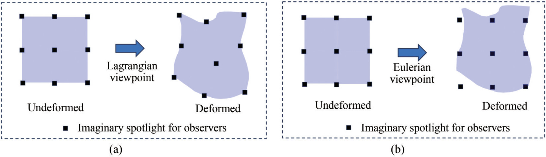Figure  1  Comparison of Lagrangian and Eulerian descriptions

Download: Full-Size Img

Inherent to the study of material motion and deformation, numerical methods serve as indispensable tools for prediction and analysis. These methods naturally fall into two categories: Eulerian methods, shown in Figure 2(a), and Lagrangian methods, shown in Figure 2(b). Each approach possesses the distinct advantages and disadvantages listed in Table 1, contributing substantially to the exploration of diverse engineering and scientific challenges in various fields. Recently, the merging of these two descriptions, harnessing their respective strengths, and the development of numerical techniques characterized by exceptional precision, efficiency, stability, robustness, and adaptability have garnered considerable attention. This paper takes three description methods—Lagrangian, Eulerian, and the coupled Lagrangian–Eulerian approach—as its foundation and delves into the current state of development and prospective applications of coupled Lagrangian–Eulerian numerical methods in the realm of ocean engineering.

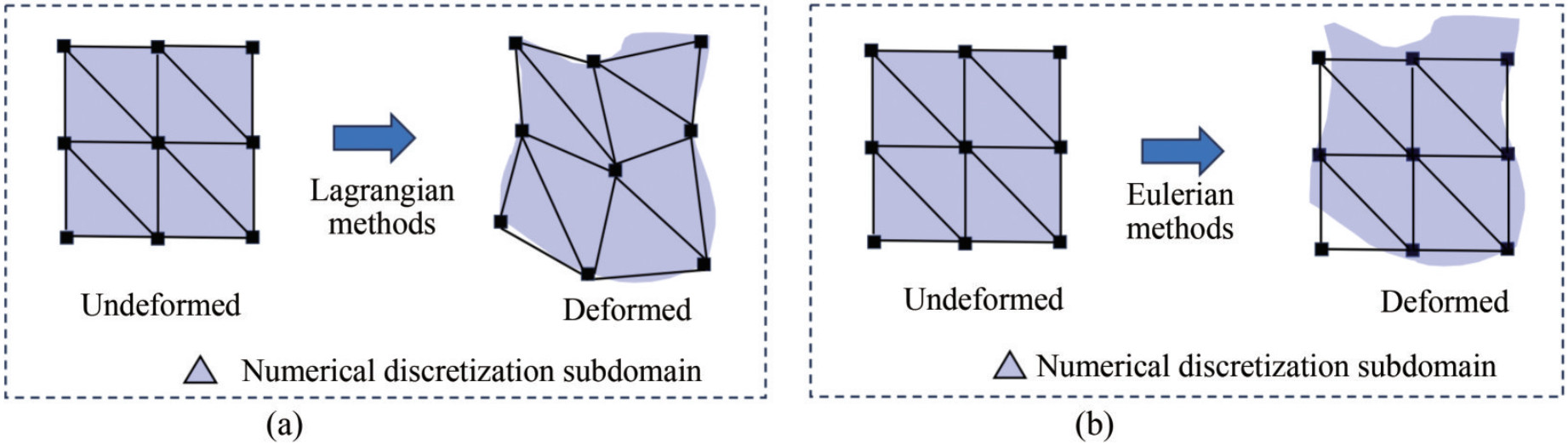Figure  2  Discretization comparison of Lagrangian and Eulerian numerical methods

Download: Full-Size Img

3.1   A brief review of the lagrangian description

In the Lagrangian description, the discretization covers the material region during the real-time simulation, as shown in Figure 3. Thus, the mesh or particles move and deform with the fluid, and the trajectory can be explicitly obtained. These characteristics of Lagrangian description are listed in Table 1 and are detailed as follows:

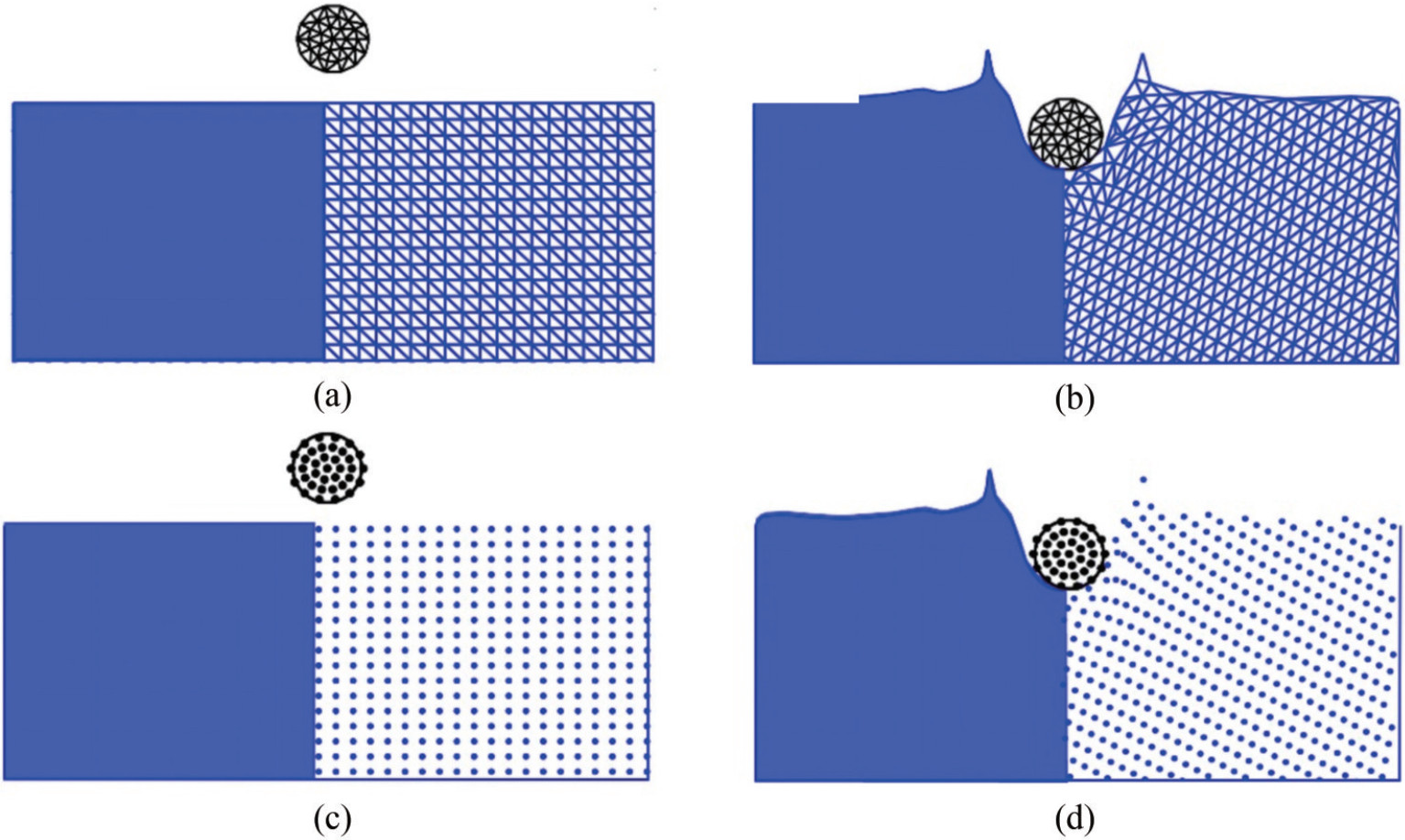Figure  3  Typical Lagrangian description in the mesh-based and mesh-free particle methods: (a) & (b) are Lagrangian meshes in the problem of a cylinder dropped into water. (c) & (d) are Lagrangian particles in this problem

Download: Full-Size Img

• Explicit tracking of fluid motion and deformation. In the Lagrangian framework, the numerical model directly tracks the particles that move with the fluid. Consequently, the particle trajectories and interactions can be accurately captured even when large deformations occur.

• Adapting to complex geometric and topological changes. For problems involving fracture, merger, phase separation, etc., which involve complex geometric and topological changes, the Lagrangian method can adapt to these changes because the topology of the discretization system is adaptive.

• Easy-to-capture surfaces and interfaces. Because each particle or grid cell represents a part of fluids, the dynamic complexity of the interface can be directly modeled by the motion of the particles without the need for special interface tracking algorithms.

• Computationally expensive. Lagrangian methods require tracking the trajectory of grids or particles, particularly when large-scale or three-dimensional flows are simulated, and this process is computationally intensive. In addition, because of the change in mesh and particle positions, the shape function must be constantly reconstructed, considerably increasing the computational effort.

• Numerical diffusion. In sparse regions of the grid or particles, the particle/node spacings become wide, reducing the accuracy of the approximation. Moreover, each particle trajectory is computed independently, and any small numerical error will accumulate while iterating the particle motion, eventually leading to diffusion in the entire flow field.

• Mesh distortion. Large deformations, fluid – structure interactions, or highly nonlinear flows can result in mesh distortion in the Lagrangian description, reducing the volume of mesh elements to near-zero or even negative values. The presence of elements with negative volume constitutes a severe numerical issue, often leading to simulation failure.

3.2   A brief review of the eulerian description

As shown in Figure 4, the Eulerian description is based on spatial or fixed coordinates. Fields (e.g., velocities and pressures) are described at fixed spatial points in the domain without the need to track individual particles. This strategy endows numerical methods based on this description with the following advantages.

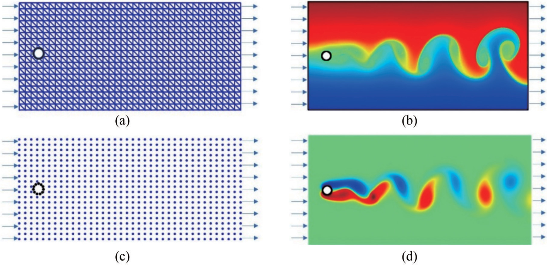Figure  4  Typical Eulerian description in the mesh-based and meshfree methods: (a) & (b) are Eulerian meshes in the problem of the flow past a circular cylinder; (c) & (d) are Eulerian nodes in this problem. (Subfigure (b) and (c) are reproduced from Qian et al. (2022), Copyright (2022), with permission.)

Download: Full-Size Img

• Easily imposed solid boundary conditions and captured boundary layer flow. In the Eulerian framework, fluid boundaries are predefined and fixed on the mesh, which allows boundary conditions to be directly and explicitly imposed on mesh points. This clear geometric representation simplifies and streamlines working with fixed boundaries. For viscous fluids, flow velocity gradients near fluid boundaries are large and must be handled carefully to properly capture boundary layer effects. Eulerian methods can improve the resolution of the solution by performing mesh refinement near the boundary to capture the boundary layer flow more accurately.

• Low computational effort and data storage. The fixed mesh does not deform with fluid motion, which reduces the need for dynamic mesh maintenance, such as mesh remapping or adaptive mesh techniques, which are necessary for Lagrangian methods. In addition, the fixed mesh avoids the process of shape function reconstruction required for the deformed mesh, further demonstrating the advantage in efficiency. Moreover, the Eulerian method has a simple data structure, regular and predictable memory access patterns, facilitating computational architectures such as vectorization and efficient cache utilization, thus improving computational efficiency.

• Easy-to-couple turbulence models. Eulerian methods facilitate the natural integration of turbulence models, such as the Reynolds-averaged Navier – Stokes (RANS) model and the Large eddy simulation (LES) model. These models are readily implemented within the Eulerian framework, as they are typically formulated based on averaged flow properties over fixed control volumes. Moreover, Eulerian methods enable accurate imposition of turbulence boundary conditions, particularly near solid walls, which is crucial for simulating wall-bounded turbulence and accurately calculating wall shear stresses.

• Easy-to-implement parallel computing. The fixed grid is well-suited for parallel computation, and memory access patterns are typically regular and sequential, facilitating efficient cache utilization and memory bandwidth on CPUs and GPUs. In parallel computing, a fixed grid can be easily partitioned into multiple subdomains, which can be evenly distributed across the multiple cores of CPUs or GPUs. This distribution helps achieve good load balancing and reduces the need for inter-processor communication, thereby enhancing overall computational efficiency.

• Additional tracking techniques for surface and interface. Eulerian methods require additional algorithms, such as volume-of-fluid (VOF) (Hirt and Nichols, 1981) and level set (Olsson and Kreiss, 2005), to identify surfaces and interfaces, thereby increasing complexity. Moreover, interface tracking techniques in Eulerian frameworks lead to numerical diffusion, resulting in blurred interfaces, particularly over prolonged simulation durations. This diffusion poses considerable challenges in accurately depicting sharp interfaces, in contrast to Lagrangian methods, where the particle or grid positions directly correspond to interface locations.

• Grid-related issues. When fluids experience overturning and fragmentation, the local scale of the flow field can be substantially diminished compared to the local grid scale, leading to an inability to capture fine details and causing numerical diffusion. Moreover, fixed grids often poorly accommodate drastic morphological changes in materials, such as interface fracturing and merging. This inadequacy results in a coarse approximation of interfaces and a decrease in accuracy.

3.3   Coupled lagrangian–eulerian description

Because Eulerian and Lagrangian descriptions have different advantages, the coupled Eulerian–Lagrangian approach is proposed for combining the advantages of both descriptions. As shown in Figure 5(a), the coupled Lagrangian – Eulerian methods can be broadly divided into two categories. The first category is the ALE method. The grid based on the ALE method can be fixed to the material or to space. Its movement is determined based on the requirements. For instance, the ALE grid is often fixed to the material for interface tracking near free surfaces and fluid–solid interfaces, whereas it can be fixed to space to avoid grid distortion inside the fluid domain. The ALE method flexibly uses different descriptions at different times and locations, effectively combining the strengths of the Lagrangian and Eulerian descriptions.

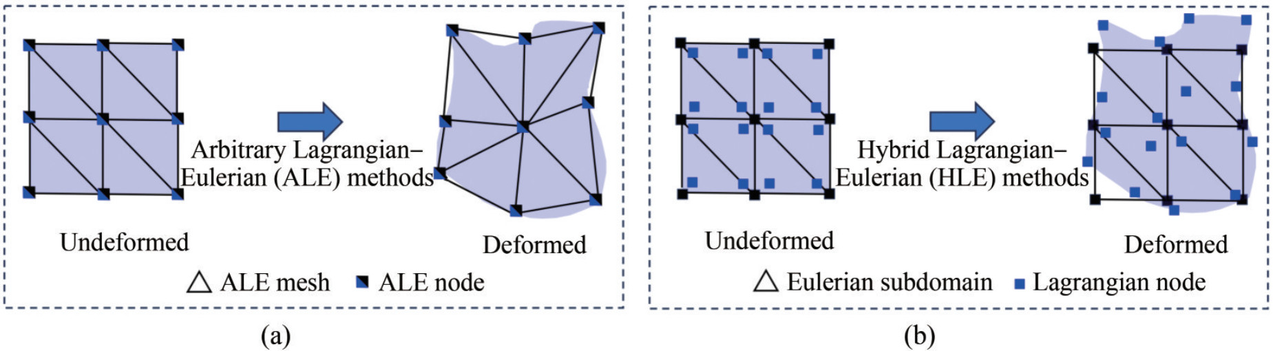Figure  5  Two types of Lagrangian–Eulerian coupled descriptions

Download: Full-Size Img

The other category is the HLE method, as shown in Figure 5(b), which simultaneously uses both descriptions in the same location. The Eulerian grid/nodes are fixed in space to solve governing equations, while the Lagrangian grid/particles are fixed to the material to describe material deformation and movement. Information is transferred between the two descriptions through interpolation. This feature allows for efficient tracking of interface movement and deformation using the Lagrangian grid/particles while avoiding grid distortion by fixing the Eulerian grid. Additionally, the fixed Eulerian grid eliminates the need for reconstructing shape functions and stiffness matrices during computation, considerably enhancing computational efficiency.

To illustrate the strengths and weaknesses of the ALE and HLE methods in ocean fluid dynamics simulations, this paper will compare their computational processes and performances in typical application scenarios using the ALE-FEM, the PIC method, the MPM, and the LESCM as representatives. A comparison of these methods in various aspects will be elaborated on in the following sections and is briefly outlined in Table 2.

4   ALE method

In computational fluid dynamics, the ALE (Noh, 1963) method has emerged as a groundbreaking computational strategy, blending the best of the Lagrangian and Eulerian approaches. This method is highly effective in handling intricate physical processes, particularly those characterized by substantial deformations and interactions between fluid and structure. The ALE method uses a mesh that is neither permanently situated in space nor rigidly attached to any material. Instead, as shown in Figure 6, this mesh is dynamically adjusted as needed, making it exceptionally capable of large deformation. The execution of a typical ALE simulation encompasses a tripartite procedure:

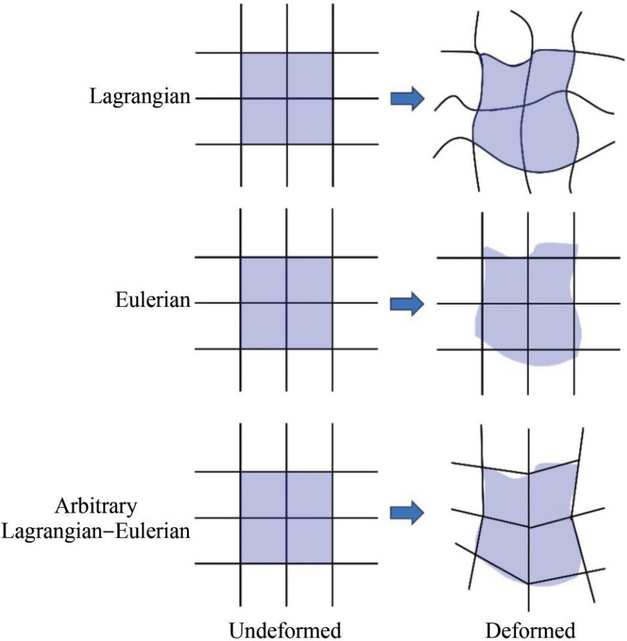Figure  6  Mesh comparison between the Lagrangian, Eulerian, and arbitrary Lagrangian–Eulerian schemes

Download: Full-Size Img

1) An explicit Lagrangian step where updates are applied to the solution and the grid.

2) A rezoning step that establishes a new grid.

3) A remapping step where the solution from the Lagrangian step is meticulously interpolated onto the new grid.

4.1   Brief introduction to ALE methods

The ALE method has yielded considerable accomplishments and fruitful results within computational fluid dynamics. Hence, following an introductory overview of the implementation process of the typical ALE method, we conduct a detailed review of two crucial techniques within the ALE method: the mesh update and mesh remapping techniques. In essence, these two techniques are the very core of the ALE method, and this section aims to elucidate their development and achievements.

4.1.1   Typical ALE formulation

On the basis of the ALE concept, researchers have proposed methods for simulating incompressible fluids using the ALE method. For a very detailed illustration, please see Yang et al. (2023) and Qing et al. (2024). Among these methods, the method proposed by Hughes et al. (1981) is representative. They introduced an ALE technique for simulating incompressible viscous flows and fluid – structure interactions, particularly in scenarios involving free surface flows.

In this section, we provide a concise overview of the principles behind ALE and briefly illustrate its implementation in computational fluid dynamics. We employ the FEM to exemplify this implementation. Initially, because the grid is subject to arbitrary motion, we introduce the state of the grid, characterized by the velocity v_g, which obtains the evolution equation of physical property Φ as follows:

where DΦ/Dt represents the material derivative, Φ_{, t} signifies the time derivative with stationary coordinates in the reference domain, c denotes the convective velocity, v is the fluid velocity, and v_g is the mesh velocity. The mesh velocity is v_g = 0 in the Eulerian framework and equates to the fluid velocity v_g = v, rendering c equal to zero in the Lagrangian framework.

In the ALE approach to fluid dynamics, consider a domain Ω ∈ Rⁿ where n equals 2 or 3, representing the space occupied by fluids. The material derivative of the fluid velocity can be represented as:

Substituting Eq. (10) into Eq. (1), the mass and momentum conservation for fluids are expressed in the ALE framework as follows:

where ρ denotes the fluid density, and p represents the pressure. The relationship between fluid pressure and fluid stress can be defined as:

in which I is the identity tensor, and the boundary conditions are established as:

in which T_g signifies the part of the boundary where the velocity is predetermined. The stress-related traction boundary conditions applied to the other parts of the boundary are represented as:

Finally, the initial condition sets a velocity field v₀(x) at t = 0 as follows:

The weak integration formulation for the FEM is:

in which q and w are the weight functions for the pressure and velocity, respectively. Then, Eq. (16) is transformed by applying the Gauss theorem (Fourestey and Piperno, 2004). Next, the discretized equations are solved using the classic finite element formulation (Filipovic et al., 2006).

For the fluid – structure interaction simulation, the finite element weak form of governing Eq. (4) for solids can be derived similarly. Furthermore, the partitioned approach (Wall et al., 2007) is applicable to the interaction. For concision, the specifics of this process are not duplicated here.

Generally, when using the ALE-FEM method to solve incompressible flow, the primary computational process in a single time step is illustrated in Figure 7(a) and described as follows:

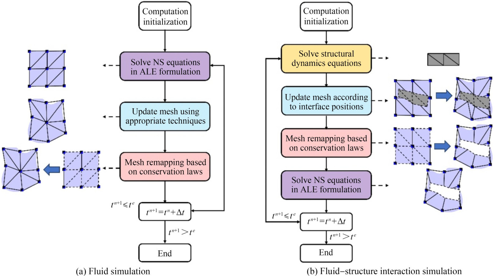Figure  7  Flow chart for a fluid simulation and fluid – structure interaction simulation based on the ALE technique

Download: Full-Size Img

1) Resolve the NS equations: Given the fluid pressure and velocity fields at time step n, the Navier–Stokes (NS) equations are solved to obtain the velocity and pressure at time step n + 1.

2) Update the mesh: The mesh is updated through mesh movement or reconstruction, yielding the displacement and velocity of the mesh nodes.

3) Mesh remapping: Under the conservation of mass, momentum, and energy, the physical quantities (such as velocity and pressure) from the old mesh are mapped onto the new mesh.

When employing the ALE technique to solve fluid – structure interaction problems, a common approach is to use a partitioned method, which involves separately solving for the fluid and solid regions. The main computational steps are shown in Figure 7(b) and described as follows:

1) Solid solution: Given the fluid pressure and velocity fields at time step n, along with the structure's displacement, velocity, and acceleration, the structural dynamics equations are solved to determine the structure's displacement, velocity, and acceleration at time step n + 1.

2) Mesh update: The interface between the structure and fluid is treated as the boundary for the fluid region. The fluid mesh is updated using mesh movement or reconstruction algorithms, calculating the displacement and velocity of the mesh nodes.

3) Mesh remapping: Under mass, momentum, and energy conservation, the physical quantities (such as velocity and pressure) from the old mesh are mapped onto the new mesh.

4) Flow field computation: The fluid motion equations are solved on the new mesh to obtain the fluid's pressure and velocity fields at time step n + 1, and forces such as drag and lift acting on the structure are calculated.

4.1.2   Progress of the mesh update algorithm

To solve ocean fluid – structure interaction problems using the classical ALE method, the mesh must be deformed in the second step to accommodate moving or solid boundaries. The quality of the deformed mesh considerably impacts the accuracy of the subsequent solution, thus highlighting the crucial role of mesh update algorithms within the ALE method. For effective mesh deformation, three fundamental criteria must be met: (1) the boundary- and interface-fitted property, (2) the prevention of grid distortion, and (3) the maintenance of overall grid quality. Furthermore, mesh update algorithms are generally categorized into physical analogy, mesh smoothing, and interpolation methods. Each of these methods is detailedly reviewed as follows:

4.1.2.1   Physical analogy methods

Physical analogy in mesh deformation methods equates the motion of grid points to various physical processes, leading to a range of mesh deformation techniques. Kennon et al. (1992) developed the flow analogy method, viewing grid point movement as fluid particle flow, which successfully updates two-dimensional unstructured grids in several sceneries.

Alternatively, Batina (1990) proposed the spring analogy technique, treating the connection between grid nodes as spring connections and updating the positions of grid nodes accordingly. However, this method primarily focuses on spring stretching and shows limited resistance to torsional deformation of the mesh. Piperno et al. (1995) proposed a two-dimensional grid torsion spring method, improving the resistance to torsional deformation. Unfortunately, this method assumes small deformations of materials and is unsuitable for cases with large deformations or small grid scales near boundaries. Blom (2000) introduced boundary correction to the spring analogy technique, increasing the spring stiffness in grid layers near moving boundaries to redistribute deformation to more distant areas, thereby improving mesh adaptability near boundaries. Overall, the stiffness matrix derived from the spring analogy method (Yang et al., 2021), characterized by diagonal dominance, is straightforward to solve but has restricted applicability.

Tezduyar et al. (1992) developed the solid analogy method for mesh deformation, where grid node displacement is determined by solving governing equations related to elastic problems. This method was further improved by Chiandussi et al. (2000); Smith and Wright (2010); Smith (2011), and Karman Jr et al. (2006), who enhanced its capabilities by adjusting parameters such as the elastic modulus and Poisson's ratio distribution, incorporating source terms, and thereby improving grid deformation potential. Furquan and Mittal (2023) employed the solid analogy method in the mesh update process in analyzing the vortex-induced vibration and flutter behind a circular cylinder. The solid analogy method, applicable to any grid type, possesses stronger deformation capabilities compared to the spring analogy method. However, its complexity and high computational demand pose challenges for large-scale applications.

4.1.2.2   Mesh smoothing methods

mesh smoothing methods, particularly those based on partial differential equations, are extensively utilized in grid deformation related to ALE methods. Löhner and Yang (1996) achieved grid velocity smoothing by solving the Laplace equation and introduced a variable diffusion coefficient. This adaptation allowed smaller grids to undergo less deformation and larger grids more, enhancing the adaptability to various grid sizes. For problems containing moving boundaries, they developed a distribution function for the diffusion coefficients to improve grid deformation and reduce the CPU times of grid reconstruction. Lomtev et al. (1999) implemented a similar approach with further enhancements. Calderer and Masud (2010) and Hussain et al. (2011) applied the Laplace equation to smooth the grid position, employing a diffusion coefficient dependent on grid cell volume. Wang and Hu (2012) used double-harmonic and double-elliptic equations for grid deformation. Although these partial differential equation-based grid smoothing methods resemble elastic body methods, they require a higher computational load.

4.1.2.3   Interpolation methods

Interpolation-based mesh update methods use known grid boundary conditions to interpolate the positions of internal points. Structured grids can employ the algebraic, polynomial, or spline interpolation method to transfer boundary displacements. In contrast, unstructured grids often necessitate explicit interpolation methods, such as point-to-point methods based on boundary distances. These methods are adaptable to various grids and have low memory requirements and high computational efficiency. Researchers such as Allen (2006), Liefvendahl and Troëng (2007), and Persson et al. (2009) have experimented with different interpolation functions and distance-based methods. The inverse distance-weighted (IDW) interpolation, a scattered data interpolation technique, was first used for grid deformation by Witteveen (2010). Luke et al. (2012) enhanced the IDW algorithm and employed the tree-code algorithm for parallel computing in large-scale grid deformation problems. De Boer et al. (2007) adopted radial basis function interpolation for dynamic grid deformation, while Rendall and Allen (2009) introduced a boundary point reduction algorithm, considerably reducing the computational burden by decreasing the size of linear equation systems.

4.1.3   Progress of the mesh remapping algorithm

The remapping of key physical quantities such as density, momentum, and internal energy from old to new grids plays a vital role in the ALE method. This process is crucial for maintaining the algorithm's accuracy and convergence. Typical methods for this process include the intersection mapping method (Powell and Abel, 2015) and the flux mapping method (Garimella et al., 2007), both of which play an important role in ensuring the effective and accurate transition of these physical quantities in the ALE method.

The intersection mapping method involves performing intersection operations between the new and old grids. This process results in numerous intersection regions. Physical quantities on these intersection regions are then aggregated into each new grid cell to derive the physical quantities on the new grid. The main advantage of intersection mapping is that it does not require the topological structures of the new and old grids to be identical, offering considerable flexibility and convenience in mesh update algorithms. The flux mapping method distinguishes itself from intersection mapping by not necessitating the calculation of intersecting points between new and existing grids, thus bypassing complex geometrical computations. This method primarily focuses on constructing flux polyhedra by assessing spatial relationships between consecutive grid cells. Following this assessment, it calculates the mass and momentum within these polyhedra, which aids in deriving the physical parameters for the updated grid. Importantly, for this approach, the new and former grids must possess identical topological structures and precise alignment. Additionally, flux mapping faces challenges in accurately determining the composition of different media within the flux tetrahedron, particularly in multiphase flow scenarios. Such limitations are important when implementing flux mapping in multiphase ALE methods, potentially leading to issues such as the creation of nonphysical material fragments, a phenomenon documented by (Kucharik and Shashkov, 2014).

Because of the limitations of both methods, some approaches combine the strengths of flux and intersection mapping (Berndt et al., 2011; Kucharík and Shashkov, 2012). These hybrid methods employ flux mapping within the material and intersection mapping near the material interface.

4.2   Applications in ocean engineering

The ALE method is widely used in fluid dynamics and fluid – structure coupling modeling (Hou et al., 2012; Souli and Benson, 2013). Because of space constraints, this article will only review and comment on the following applications:

• Ocean current modeling, encompassing its generation, dynamic movements, and interactions with physical barriers.

• Ocean wave modeling, including regular waves, irregular waves, and focused waves.

• Interaction analysis of ocean flow and offshore structures, such as ocean flow and ship interactions.

• Multiphase flow simulation, such as liquid and gas interaction and bubble dynamics.

Ferrand and Harris (2021) used the ALE method in fluid flow studies within cylindrical valves and standing wave modeling, demonstrating its applicability in designing marine structures and protecting coastlines. Additionally, Battaglia et al. (2022) studied three-dimensional sloshing models using the ALE method, emphasizing its accuracy in simulating fluid flows. Expanding the ALE method's utility, Zhu et al. (2020) employed it to simulate free surface flows around complex geometries, as demonstrated in Figure 8. They integrated advanced techniques to enhance the method's efficiency in fluid – structure interactions, pivotal for understanding the effects of ocean currents on coastal infrastructure.

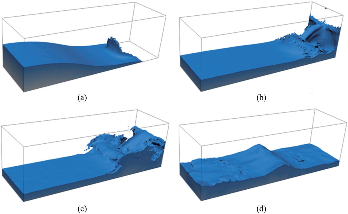Figure  8  Sequential subplots of a dam break simulation using the ALE method at time intervals t = 0.50 s, 1.25 s, 1.75 s, and 4.75 s (the results are reproduced from Zhu et al. (2020), with permission.)

Download: Full-Size Img

Wang and Guedes Soares (2016) adeptly applied the ALE method in their comprehensive analysis of stern slamming impacts on marine vessels, with an emphasis on chemical tankers. Incorporating the modified Longvinovich model, their study delved into the varied slamming loads experienced by these vessels under different sea states. Their approach, involving a detailed nonlinear time domain numerical process, provided profound insights into vessel dynamics under extreme wave conditions, highlighting the ALE method's capability in simulating complex maritime phenomena. Complementary to this study, Wang et al. (2021a) thoroughly evaluated the numerical uncertainties in the discretization of the ALE method, a crucial study that enhances understanding of force prediction and structural response accuracy in diverse maritime scenarios. Such insights are invaluable for improving the reliability and robustness of maritime structures. In naval defense, particularly regarding submarine survivability against underwater explosions, the application of the ALE method (Kim and Shin, 2008) has been groundbreaking, accurately simulating fluid – structure interactions essential for assessing and ensuring the post-attack structural integrity of submarines. This application underlines the ALE method's versatility and effectiveness in tackling complex engineering challenges.

The interaction between ocean currents and coastal structures is a critically important area of study. The ALE method has proven to be an indispensable tool in this field. Xiang and Istrati (2021) employed the ALE method to model the effects of solitary waves on open-girder bridge deck geometries, providing substantial insights, as shown in Figure 9. Their research illuminates the influence different girder numbers and varying wave heights have on wave-induced forces, contributing to the understanding of coastal structure resilience in extreme wave conditions. Piperno et al. (1995), Piperno and Farhat (2001) proposed a weak coupling technique that facilitates using existing fluid and structure solvers for fluid – structure coupling problems by simply transferring interface data between solvers. This technique enables the direct coupling of numerous advanced numerical methods for simulating marine fluid – structure interactions. However, this approach proves insufficient in cases of strong coupling between fluid and structure. Addressing this issue, Hübner et al. (2004) developed a strong coupling method, providing an integrated solution for fluid and structure interactions and thus removing the limitations of weak coupling. In parallel, Huerta and Liu (1988) expanded the Petrov – Galerkin FEM within the ALE framework, focusing on its application in complex fluid – structure challenges such as dam breaks and substantial fluid sloshing. Furthermore, Peery and Carroll (2000) introduced the multi-material ALE (MMALE) method, which overcomes the traditional ALE method's limitation of a single material per cell by employing mixed meshes. This approach integrates interface tracking and reconstruction algorithms (Hirt and Nichols, 1981; Rider and Kothe, 1998; Chen et al., 2017b) to effectively manage large deformations, including twisting, fracturing, and merging of interfaces, thereby enhancing the simulation of intricate oceanic flows.

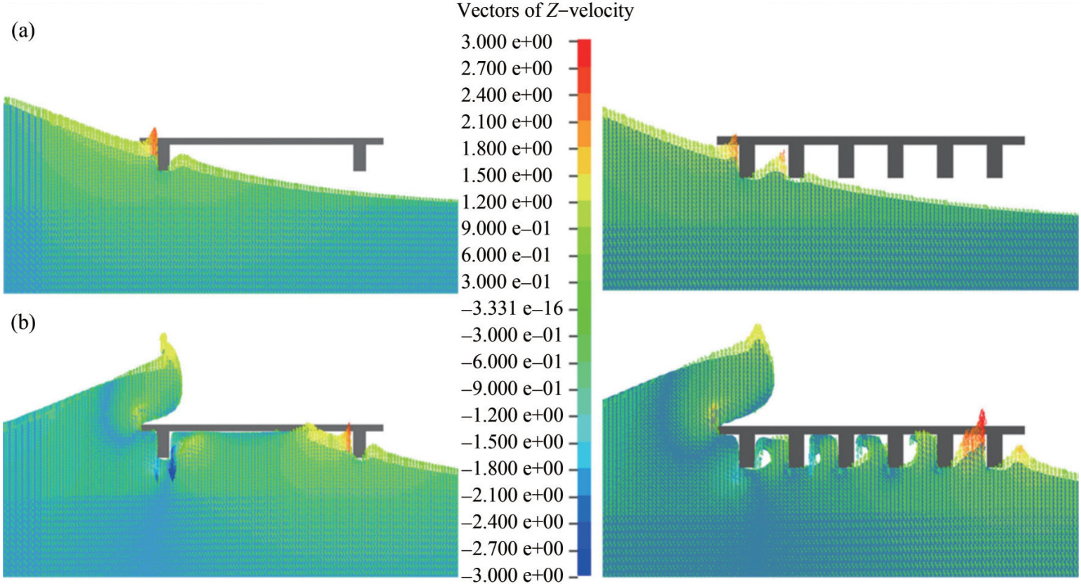Figure  9  Snapshots of fluid velocity depicting water waves impacting a deck with two beams (left) and six beams (right) at time points (a) t = 6.2s and (b) t = 6.5s, as simulated by the ALE method (the results are reproduced from Xiang and Istrati (2021), with automatic permission granted under the open-access policy)

Download: Full-Size Img

Bubble dynamics involves issues of damage and protection of ships and marine structures and has increasingly attracted researchers' attention in recent years. Zhang et al. (2023) proposed a unified theory of bubble dynamics that provides an important theoretical basis for high-accuracy analysis of bubble problems. Inspired by this study, Gao et al. (2023) used the ALE method to analyze the damage characteristics of the cabin in a navigational state subjected to a near-field underwater explosion, considering the effects of asymmetric bubble collapse and accurately predicted the cavitation erosion risk areas. Using the ALE method, Jia et al. (2019) investigated the free-rising bubble with mass transfer, finding that the thickness of the concentration boundary layer dominates the mass transfer behavior at the bubble surface.

Overall, these studies collectively emphasize the ALE method's exceptional adaptability and precision in simulating complex fluid – structure interactions, reaffirming its vital role in advancing ocean engineering and enhancing maritime safety and structural resilience.

4.3   Current merits and shortcomings

The ALE method skillfully combines the Lagrangian and Eulerian methods, offering the following advantages:

• Improvement of mesh distortion. The ALE method enables the mesh to be defined flexibly and tailored to the deformations and motions of fluid and structure. This adaptability effectively alleviates the issue of mesh distortion commonly encountered in Lagrangian meshes.

• Enhanced tracking of interfaces and free surfaces. Nodes near interfaces and free surfaces can be fixed accordingly to fluids and structures and move with them. This feature ensures accurate tracking of fluid – structure interactions and the dynamics of free surfaces.

Because of the characteristic of the ALE mesh to move freely, it solves the mesh distortion problem found in the Lagrangian method while addressing the difficulty in capturing moving interfaces inherent in the Eulerian method. Thus, the ALE method overcomes the disadvantages of both descriptions by combining their concepts, making it an effective algorithm for simulating oceanic fluid – structure interaction problems, and it has been widely applied and developed over the years. However, it also inherits disadvantages from both methods, as follows:

• Issues of accuracy and stability. Mesh movements that violate the geometric conservation law (Thomas and Lombard, 1978) can lead to the inability to maintain uniform flow and computational instability. Although Thomas and Lombard (1979) proposed techniques to improve geometric conservation, this issue remains important in complex fluid – structure interaction simulations.

• Temporal discretization limitations. Étienne et al. (2009) observed that time discretization schemes with p-order accuracy on a stationary grid may not maintain the same accuracy when applied to a dynamic ALE mesh.

• Mesh reconstruction limitations. As noted by Baiges et al. (2017), the ALE method necessitates continuous deformation and reconstruction of the computational mesh. This process is not only resource intensive but also struggles to ensure high-quality meshes in intricate fluid – structure interaction scenarios.

Because of the limitations of the ALE method, particularly the complexity of mesh reconstruction, its application to large-scale, three-dimensional engineering problems has been challenging. Scholars continue to explore and seek to develop a numerical method that combines the advantages of the Lagrangian and Eulerian descriptions while eliminating the need for mesh reconstruction. Consequently, the PIC method with a hybrid Lagrangian – Eulerian description has been developed.

5   Particle-in-cell method

The PIC method was developed by Harlow (1964). As shown in Figure 10, the PIC method employs an Eulerian grid to compute governing equations and discretizes fluids into particles, and each particle is characterized by mass, momentum, and energy. In simulations, particles traverse the Eulerian grids, representing the motion and deformation of fluid. The PIC method primarily involves two computational steps:

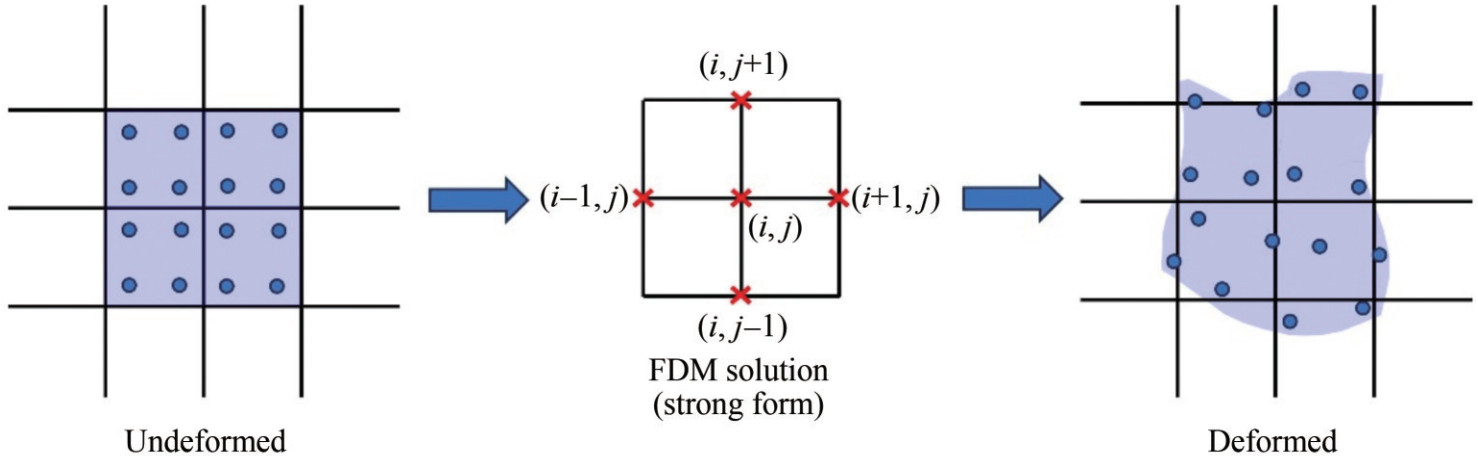Figure  10  Hybrid Lagrangian–Eulerian description in the PIC method

Download: Full-Size Img

1) The transportation effects of the fluid are ignored, and Lagrangian calculations are directly performed using the finite difference method (FDM) to assess changes in momentum and energy on the Eulerian grid.

2) Each particle position is determined using interpolation or mapping techniques on the Eulerian grid and then updated at the end of the current timestep.

This second step effectively addresses the fluid transportation effect disregarded in the initial calculations. In the simulation process of PIC, the grid solidifies on the material within a single time step and subsequently deforms and moves with it. This feature allows for the direct solution of the NS equations on a uniform grid. At the final stage of each time step, the grid maps the motion and deformation information onto the particles, which then carry all the flow field information. Thus, at the beginning of the next time step, the deformed grid can be discarded, and the particle information is directly mapped back to the undeformed uniform grid for continued solution. This process efficiently avoids the grid reconstruction required in the ALE method, considerably reducing the computational load of the solution process. Meanwhile, the PIC method retains the advantages of a hybrid description. The PIC concept has profoundly influenced various computational methods and has been implemented in numerous fluid dynamics simulations (Brackbill and Ruppel, 1986; Sulsky et al., 1994; Nestor et al., 2009).

The initial version of the PIC method exhibited considerable dissipation (Noh, 1963), resulting in poor accuracy and extensive memory demands, thus complicating the solution of large-scale problems. To address these issues, Gentry et al. (1966) developed the FLIC method, building upon the PIC method. FLIC is similar to PIC in its first step, using an Eulerian grid to solve equations, but differs from PIC in its second step. Rather than advecting individual particles, it shifts continuous fluid masses, computing mass transfers across grid boundaries and, subsequently, the momentum and energy transfers carried by this mass, ultimately determining each grid's new velocity and energy. Expanding on this concept, Harlow and Welch (1965) devised the MAC method for simulating incompressible free surface flow problems. The MAC method, still based on an Eulerian grid, focuses on pressure and velocity as primary variables and employs differential methods to solve the Navier–Stokes equations. Additionally, it integrates numerous massless markers within the grid, tracking each to ascertain fluid presence during computations. The MAC method has gained widespread application in free surface and multiphase flow problem computations.

The classic PIC method only retains mass and location data on particles, with other physical quantities stored on the grid. This separation results in considerable numerical dissipation during momentum transfer between the grid and particles, lowering the accuracy. Recent advancements aim to enhance PIC's accuracy: One involves the development of more sophisticated advection algorithms, while another strategy involves equipping particles with comprehensive material information throughout the simulation. The background grid acquires this information through mapping at each timestep. Building on these ideas, Brackbill and Ruppel (1986) endowed particles with complete fluid material information and developed a low numerical dissipation version of the PIC method, known as the FLIP method. This approach has achieved widespread adoption.

Recently, Kelly et al. (2015) and Chen et al. (2016a) developed the incompressible particle-in-cell (PICIN) method for simulating oceanic fluid – structure interaction problems based on an incompressible flow model and the cut-cell method. In this method, solids are treated as rigid bodies, with a layer of particles arranged on the solid surface to represent boundaries and identify fluid – structure interfaces. The rigid body is overlaid on a background grid, and the two-way coupling simulation of incompressible fluid and a six-degree-of-freedom rigid body is achieved using the cut-cell method (Tucker and Pan, 2000). Additionally, the PICIN method draws on the FLIP approach by considering acceleration and velocity on the background grid during the velocity mapping process, substantially reducing numerical dissipation. Because of its hybrid description, the PICIN method is more efficient than the purely Lagrangian SPH method. Furthermore, by introducing Lagrangian particles, the identification of fluid – structure interfaces and free fluid surfaces are efficient and accurate, enabling precise simulations of complex processes such as wave breaking and rolling. Chen et al. further incorporated MPI parallel technology to extend the PICIN method to large-scale and complex numerical simulations of ocean flow interacting with columns, achieving a series of research results (Chen et al., 2016b; 2018a; 2019b). Thus, we briefly recall the state-of-the-art PICIN formulation in this part.

5.1   Brief formulation

After years of development, the PIC method has evolved to possess a well-established framework. Comprehensive details regarding the theory and implementation procedures are found in recent research (Snider, 2001; Qu et al., 2022; Yu et al., 2023).

A typical discretization scheme (Kelly et al., 2015) of an incompressible fluid for the PIC method is shown in Figure 11. First, a staggered Eulerian grid is used in this scheme, which can effectively alleviate the checkerboard problem in the solution of the Navier – Stokes equations. Second, the Lagrangian particles initialized in each water-filled cell are introduced to describe the fluid motion and deformation.

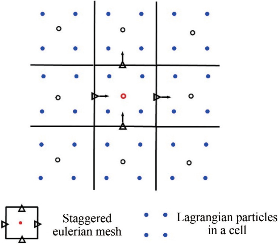Figure  11  Discretization of the computational domain in the PIC framework

Download: Full-Size Img

5.1.1   Information transfer between lagrangian and eulerian descriptions

5.1.1.1   Particles-to-mesh transformation

The Eulerian solution procedure is initiated by transferring the fluid velocity from Lagrangian particles to a staggered mesh. This transfer, which can use several types of interpolation methods, can be expressed as:

in which N_j denotes the interpolation function, which can be chosen as a kernel function (Liu and Liu, 2010; Kelly et al., 2015), finite element shape function (Qian et al., 2024), etc. m_i and $\tilde{m}_j$ represent the fluid mass associated with fixed nodes and particles, respectively. Similarly, v_i and $\tilde{\boldsymbol{v}}_j$ correspond to the velocities of nodes and particles, respectively.

5.1.1.2   Mesh-to-particles transformation

Upon completing the Eulerian stage, where the velocity solution of the NS equations is obtained, fluid data must be mapped from the mesh back to the Lagrangian particles. Several interpolation functions can be used for the mesh-to-particle transformation:

in which φ_i is selected as a weighted essentially non-oscillatory function (WENO; Jiang and Shu (1996)), kernel function (Monaghan, 1985), RK function (Liu et al., 1995), finite element shape function (Zhang et al., 2017), etc.

5.1.2   Eulerian step in the PIC framework

The Eulerian step of the typical PIC method is to apply the body force and viscous force to obtain the intermediate velocity v_f^*, which is formulated as:

in which $\boldsymbol{v}_f^n=\{u, v\}^{\mathrm{T}}$ is the fluid velocity vector at the nth step in the two-dimensional cases. Then, the viscous force can be easily computed using a simple forward-in-time centered-in-space (FTCS) difference scheme.

Although the body force and viscous force are applied using Eqs. (19) and (20), the intermediate velocity v_f^* is unlikely to be divergence-free. Therefore, the fluid pressure should then be calculated to prepare the divergence modification in the next step. The fluid pressure is obtained using the pressure Poisson equation (PPE; Chorin (1968)) as follows:

This equation can be discretized into:

Obviously, the pressure vector $\boldsymbol{p}=\left[p_1, \cdots p_n\right]^{\mathrm{T}}$ at all nodes can be calculated by solving the algebraic equations constructed by Eq. (22), which obtains:

in which A is the matrix of coefficients associated with grid size Δx and Δy, and d is the vector related to the intermediate velocity v_f^*. After obtaining the pressure vector p by solving Eq. (23), the final velocity, v_fⁿ⁺¹, can be obtained by:

and by applying the finite difference scheme, Eq. (24) can be calculated as:

5.1.3   Lagrangian step in the PIC framework

The Eulerian stage ends when the final velocity v_f is obtained through Eq. (24). Then, the Lagrangian stage that advects the particles is applied by integrating the following equation:

Here, the Runge–Kutta scheme (Ralston, 1962) or leap-frog scheme (Pan et al., 2013) is used for the particle position update. In addition, to make particle distribution as uniform as possible, particle shifting techniques (PSTs; Zhang et al. (2018b); Lyu and Sun (2022); Gao and Fu (2023)) should be employed after the particle position update.

5.2   Application in ocean engineering

PIC is a classic method that was developed several decades ago. It has been widely used in several areas (Markidis and Lapenta, 2011; Grigoryev et al., 2012). Specifically, PIC has the following successful applications in oceanography and coastal engineering:

• The dynamics of ocean waves, encompassing their generation, breaking, and interactions with structures.

• The interaction between ocean flow and coastal structures.

• The interaction between ocean flow and floating structures, encompassing ship hydrodynamics, wave generation, etc.

• Multiphase flow in ocean environments.

• Shallow water dynamics.

Recently, Kelly et al. (2015) and Chen et al. (2016a, 2019b) completed a large amount of algorithm research, simulation platform development, and applications in ocean flow and coastal engineering based on the PIC method, which has greatly contributed to the development of PIC methods in the field of ocean hydrodynamics. Initially, on the basis of the cell-cut technique, which realizes fluid – structure interaction calculations on a fixed Eulerian grid, Kelly et al. (2015) proposed the PICIN method for the two-way fluid – solid coupling scheme. For free surface flow simulations, the fast-sweeping method efficiently identifies free surfaces in ocean flows, enabling simulations of fluid – structure interactions associated with coupled ocean flow and offshore structures, as depicted in Figure 12. Furthermore, the PIC framework has been comprehensively developed for two- and three-dimensional computations in large-scale ocean flows, as illustrated in Figures 13 and 14.

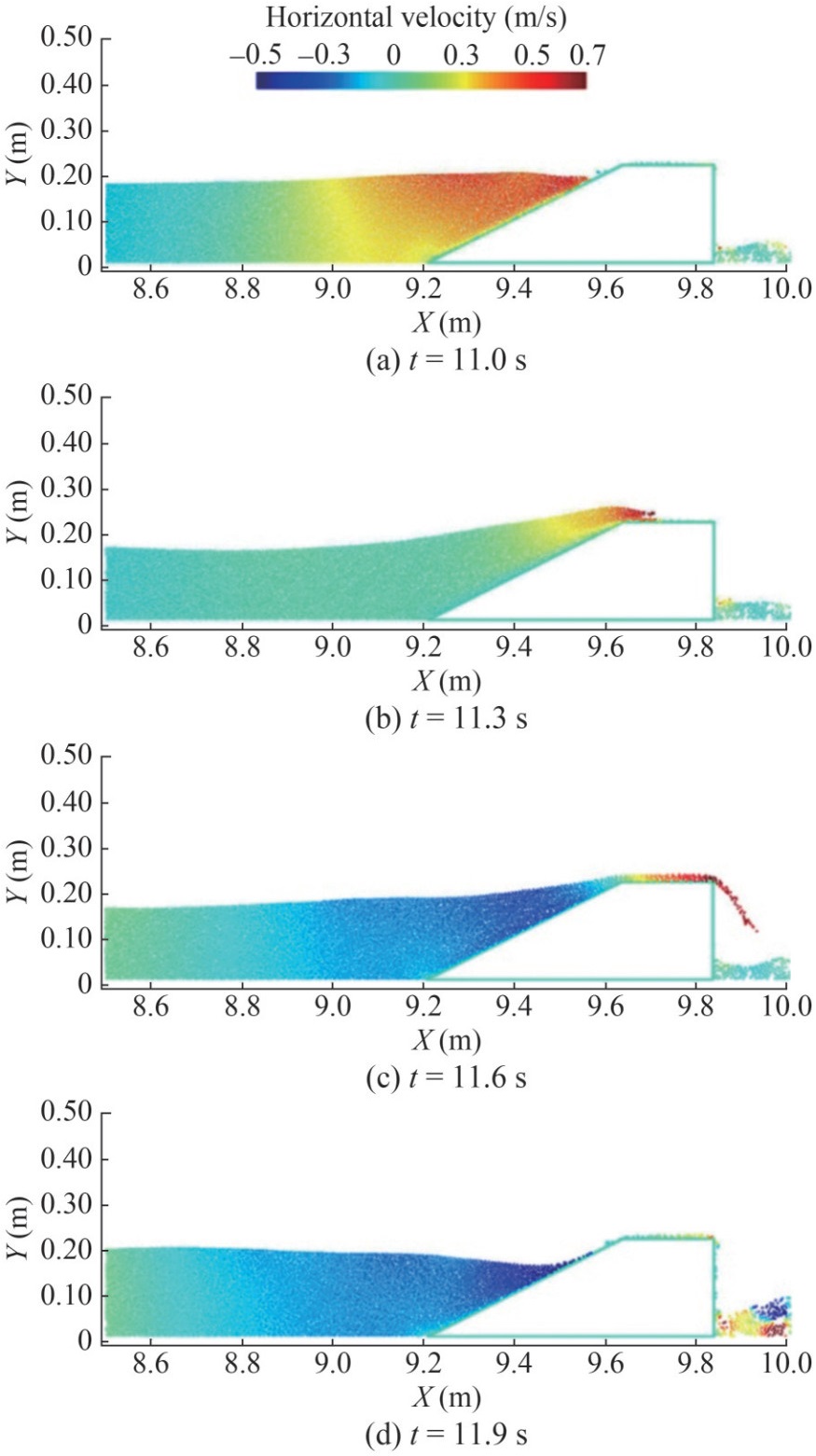Figure  12  Results from a PIC method simulation showing the wave profile and velocity field adjacent to a low-crested structure during overtopping. (The results are reproduced from Chen et al. (2016a), with permission.)

Download: Full-Size Img

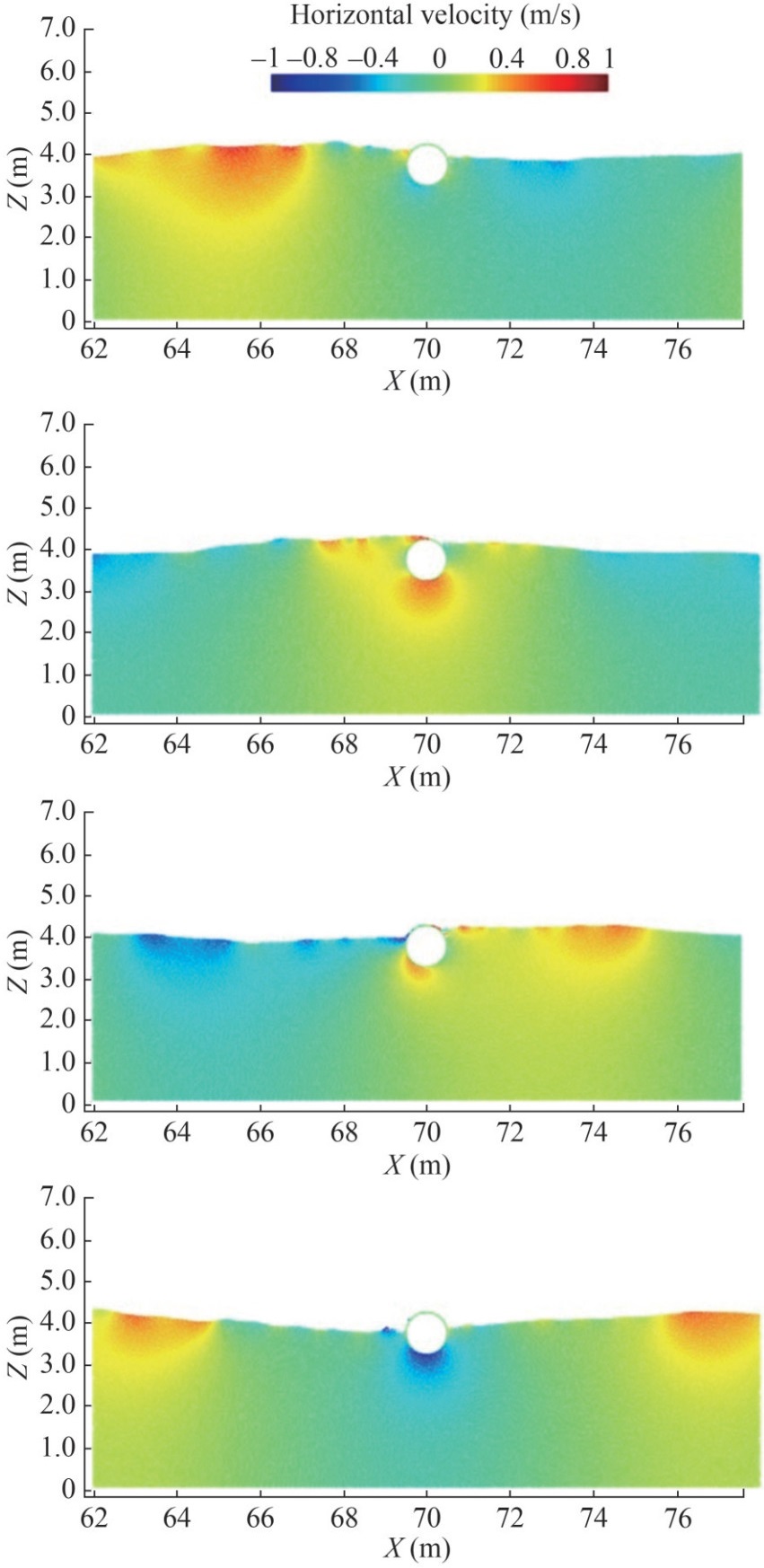Figure  13  Snapshots of wave interaction with a fixed cylinder according to the PIC method. (The results are reproduced from Chen et al. (2016b), with permission.)

Download: Full-Size Img

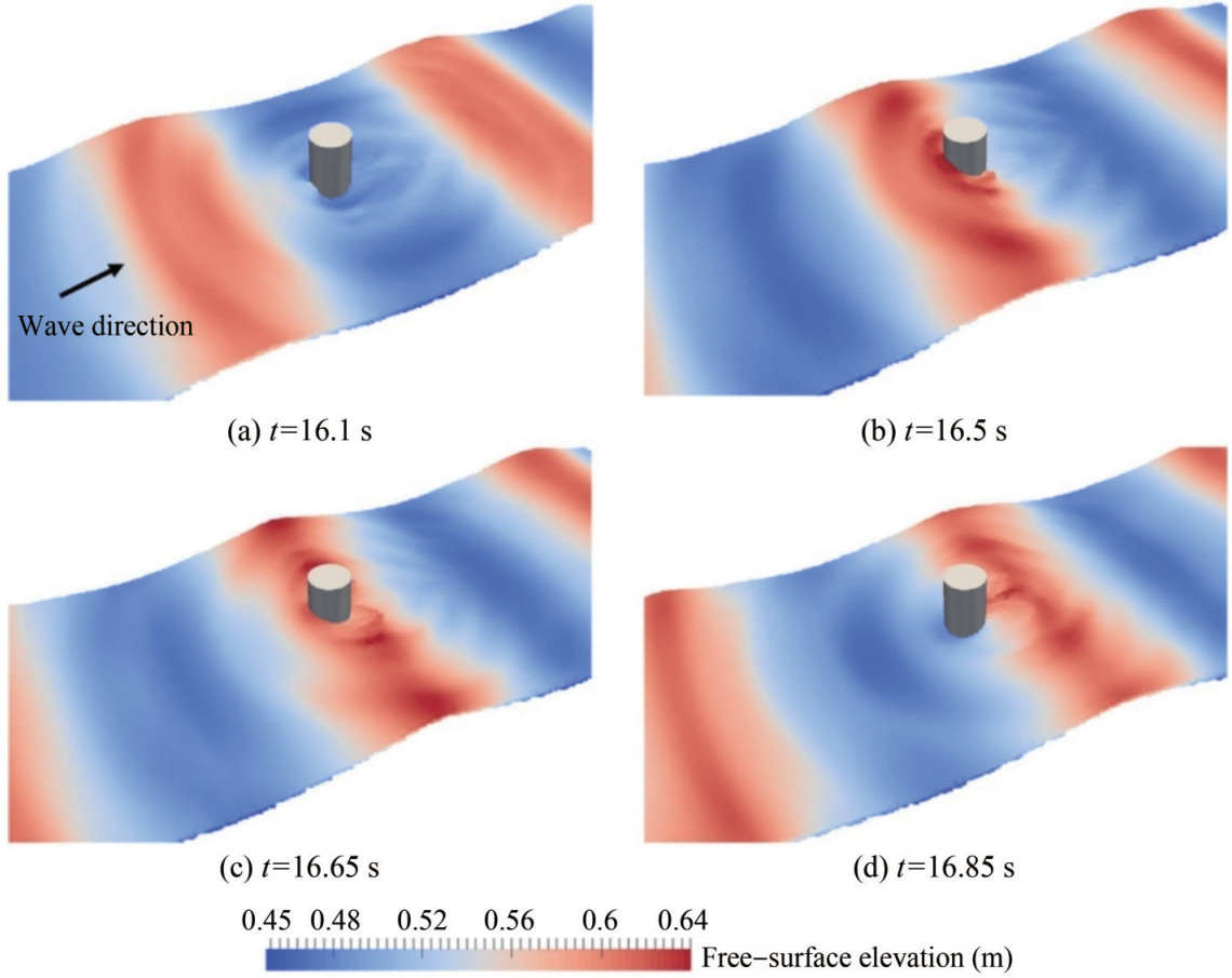Figure  14  Snapshots from the PIC method-based numerical simulation of regular wave interaction with a single cylinder. (The results are reproduced from Chen et al. (2019b), with permission.)

Download: Full-Size Img

Then, the numerical wave generation technique is introduced to the PICIN framework, and different relaxation approaches are compared for the effect of absorbing water waves in the PICIN method (Chen et al, 2019a). The results show that the modified relaxation method tends to reduce the length of the relaxation zone by approximately 50% while still achieving similar performance to that of the regular relaxation method. The dynamic behavior of the interaction between ocean flow and coastal structures is investigated using the PICIN method (Chen et al., 2016a), and several benchmarks, including wave overtopping of a low-crested structure and dam-break-induced overtopping of a containment dike, are tested.

The interaction between floating structures and ocean flow is another important issue in ocean hydrodynamics. Because the governing equations for fluid and structures are solved on the Eulerian background grid, the interaction algorithm of fluid and solid should be applied on this grid, which means the classic cut-cell technique (Tucker and Pan, 2000; Gao et al., 2007; Xie, 2022), overset technique (Tang et al., 2003), or immersed boundary method (Sotiropoulos and Yang, 2014) can be used for the interaction calculation. Kelly et al. (2015) coupled the cut-cell method to realize a two-way fluid – structure coupling calculation of the PIC method. Chen et al. (2019b, 2020) successively explored the interaction between two- and three-dimensional floating bodies and ocean flow. The numerical model was validated by comparing it to a three-dimensional experiment on the interaction of focused waves with a floating and moored buoy. Furthermore, when benchmarked against a complex scenario involving extreme wave–structure interactions, the computational efficiency of the PIC was comparable to that of the advanced OpenFOAM® model (Jasak et al., 2007).

The coupling of ocean flow with large columns or groups of columns during the construction and operation of offshore oil platforms, sea bridges, etc., is another important engineering application. This complex problem, including the dynamics of ocean currents interacting with typical single columns and column groups, can also be analyzed using the PIC method (Chen et al., 2018a). The results show that the computational efficiency of the PIC method in this problem is near that of the VOF-FVM method in the open-source software OpenFOAM (Jasak et al., 2007; Jacobsen et al., 2012), and its accuracy of computed impact forces and wave elevation agrees well with experimental and numerical results under various conditions.

The PIC method also has important applications in multiphase flows. Kumar et al. (2021) developed the MPPIC-VOF model by combining the multiphase particle-in-cell (MPPIC) method with the VOF solver to simulate particles in two-phase flows. LES turbulence modeling was employed to address gas–liquid interface issues within hydrocyclones. Using four- and two-way coupling mechanisms, they discussed the flow characteristics of particles and their impact on the fluid flow field. Then, the MPPIC-VOF model was employed to investigate the impact of solid particles on the pressure drop and void fraction in gas – liquid flows characterized by slug and plug flow patterns (Ranjbari et al., 2023). Although these PIC-based multiphase models are not currently used directly in marine engineering analyses because of their large computational cost, they have good potential for applications in ocean multiphase flows.

Because the ocean is much wider than deep, a simplified version of the NS equations, the shallow water equations (Tan, 1992; Camassa et al., 1994), is often used in analyses of ocean hydrodynamics. The PIC method is also used to solve the shallow water equations. Pavia and Cushman-Roisin (1988; 1990) adapted the PIC method to studying oceanic geostrophic fronts, offering a computationally efficient and robust solution to previously challenging oceanic problems. Cushman-Roisin et al. (2000) use a PIC method designed for analyzing shallow water dynamics in laterally confined fluid layers, with applications extending to the study of ambient rotation effects in geophysical fluids such as open-ocean buoyant vortices.

5.3   Current merits and shortcomings

The PIC method is a classic hybrid Lagrangian–Eulerian particle method with mature applications in various fields such as thermodynamics (Gannarelli et al., 2003), plasma phenomena (Chien et al., 2020), and computer graphics (Jiang, 2015). Over years of development, the PIC method now exhibits the following advantages:

• High computational efficiency. Compared to traditional Lagrangian particle methods (such as SPH (Liu and Liu, 2003), MPS (Koshizuka and Oka, 1996), and RKPM (Liu et al., 1995)) that require searching for neighboring particles and continuously reconstructing shape functions in the solution process of governing equations, the PIC method solves equations on a fixed background grid. This approach avoids the need for searching neighboring particles and repeatedly reconstructing shape functions, thus considerably enhancing computational efficiency (Kelly et al., 2015).

• Effective boundary condition implementation. The use of a fixed Eulerian grid simplifies the imposition of boundary conditions. Dirichlet and Neumann boundaries can be applied with high accuracy.

• Proficiency in handling free surfaces and interfaces: The particle movement directly reflects the fluid motion and deformation, allowing for convenient identification of free surfaces and interfaces.

• Multi-field coupling capability: The PIC method has found extensive use in diverse fields, including hydrodynamics, aerodynamics, and thermodynamics. Its application in multi-field coupled calculations has laid a substantial foundation.

The PIC method amalgamates the strengths of Lagrangian and Eulerian descriptions, facilitating efficient simulations of intricate oceanic flows. However, this method also assimilates certain drawbacks inherent to the Lagrangian and Eulerian frameworks, as detailed subsequently.

• High memory usage: The PIC method employs a dual description system (background grid and Lagrangian particles), resulting in numerous intermediate variables that must be stored during computation. This necessity leads to high memory usage in the PIC method.

• Lack of mature solutions for turbulence: The Lagrangian particles in the PIC scheme are often four times (in 2D) or eight times (in 3D) the number of fluid grid cells. To capture the details of turbulence, PIC requires a very high grid resolution, which necessitates a greater number of discrete particles, complicating the turbulence simulation.

• Difficulty in achieving a highly accurate mapping scheme: The accuracy of the mapping between particles and the grid depends on factors such as particle density, uniformity, and mapping technique. However, particle density is considerably lower near interfaces and boundaries, and uniform distribution of particles is difficult to ensure in real time during their flow. These factors limit the ability of the PIC method to achieve high-accuracy calculations.

• Theoretical challenges in addressing the pressure Poisson equation (PPE). The PIC method necessitates resolving a large system of algebraic equations related to the PPE on a background grid. When applied to large-scale and complex problems, this requirement imposes a substantial computational burden. The extensive calculations demanded by the equations present considerable challenges in terms of memory capacity and computational power, particularly for high-resolution and intricate simulations.

Using finite difference methods, the PIC method directly calculates the constitutive equations of fluids on a background grid, where these equations are independent of deformation history. However, the constitutive relations of solids often depend on their deformation history, rendering the PIC method unsuitable for simulating solid dynamics problems. Consequently, researchers developed the MPM, tailored for solid dynamics.

6   Material point method

As shown in Figure 15, Sulsky et al. (1994, 1995), building on the PIC method, adopted the finite element weak form and material point integration to compute the constitutive equations on particles. This undertaking led to the development of the MPM, enabling the coupled computation of fluids and deformable bodies. For recent developments in the MPM, see de Vaucorbeil et al. (2020) and Song et al. (2024).

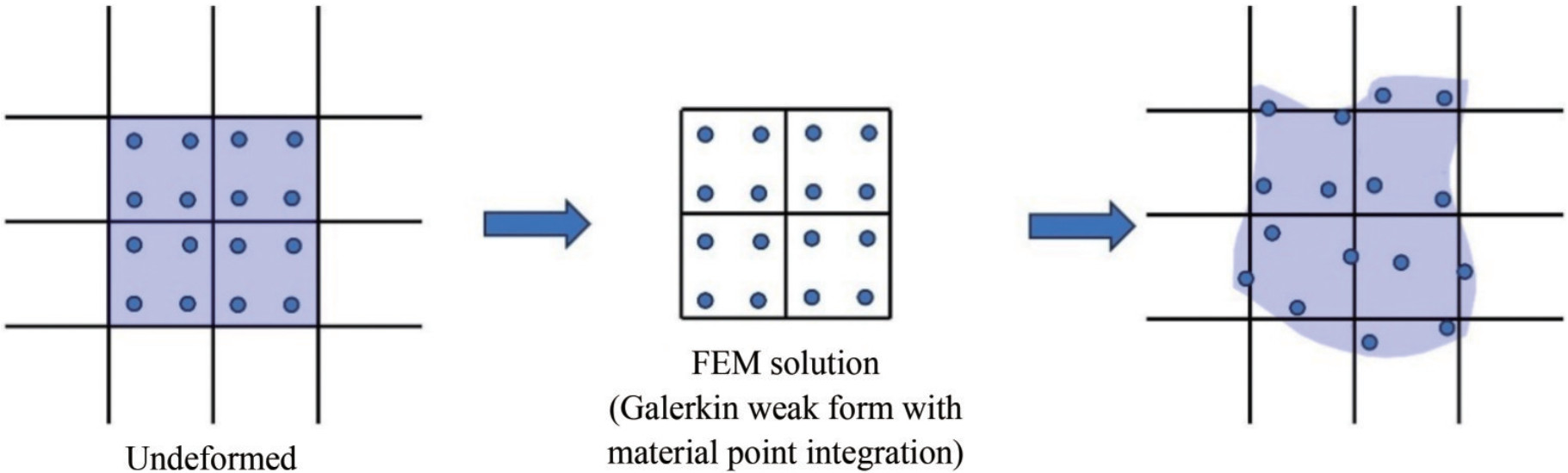Figure  15  Hybrid Lagrangian–Eulerian description in the MPM

Download: Full-Size Img

6.1   Brief formulation

To formulate the MPM, the momentum equation for fluids and solids can be summarized as the momentum equation for continuous media, which is

The boundary conditions are:

Then, for liquid flows, weakly compressible models are often used in the MPM, which means:

where p represents the fluid pressure, τ signifies the viscous stress, and I is the unit tensor. G = ρ₀c² is the bulk modulus, in which c denotes the artificial sound speed and ρ₀ the reference density. ε_V and ε denote the volumetric strain and the strain in the Voigt format, respectively. For more information on Eq. (29), see Chen et al. (2018b).

For deformative structures, the constitutive model can be formulated as follows:

in which $\hat{\boldsymbol{\sigma}}_s$ is the Jaumann stress rate, and $A\left(\dot{\boldsymbol{\varepsilon}}, \boldsymbol{\sigma}_s, \cdots\right)$ denotes the specific constitutive model for different materials.

The weak integral form of Eqs. (27)–(30) can be formulated as:

in which δv represents the test function. In the MPM, the continuum is discretized into a series of particles, as shown in Figure 15, and the density of the continuum can be approximated:

in which m_p denotes the mass of particle p, δ represents the Dirac delta function, and x_p is the coordinates of particle p. The weak integral form, Eq. (31), can be approximated as the form of material point integration by substituting Eq. (32) into Eq. (31), which gives:

where the subscripts i and j denote the components of the spatial variables that satisfy the Einstein summation convention, and $\delta v_p=\delta v\left(\boldsymbol{x}_p\right) \delta v_{i p, j}=\delta v_{i, j}\left(\boldsymbol{x}_p\right), \sigma_{i j p}=\sigma_{i j}\left(\boldsymbol{x}_p\right)$, and $b_p=b\left(\boldsymbol{x}_p\right)$. For simplicity, the traction term in Eq. (33) is omitted. Please see Remmerswaal et al. (2017) and Bing et al. (2019) for a detailed imposition of Neumann boundary conditions.

In the solution process of momentum Eq. (33), the particles and the background grid are fully coupled and move together in each time step. Consequently, finite element shape functions based on the background grid can be established as interpolation functions to facilitate the information mapping between particles and the grid. The momentum equation is then solved based on this background grid. Thus, the mapping process can be applied as:

Substituting Eq. (34) into Eq. (33) and invoking the arbitrariness of δv_iI lead to the following momentum equation on the background grid:

in which $p_{i I}=m_I \dot{v}_{i I}$ is the nodal momentum with nodal mass $m_I=\sum\limits_{p=1}^{N_p} \varPhi_{I p} m_p$. At this point, the update of momentum on the background mesh is achieved, i.e., the solution of the momentum equation is obtained.

Therefore, the solution process of the classical MPM can be summarized as follows:

1) Map the mass and momentum from particles to the grid and impose the boundary conditions on the grid; for detailed information, see Zhang et al. (2008).

2) Calculate material stress using a constitutive model.

3) Calculate the time derivative of momentum using Eq. (35).

4) Integrate the momentum equation to update the momentum.

5) Map the updated momentum from the grid to particles.

6) Update particle velocity and position and go to the next step.

6.2   Applications in ocean engineering

The MPM is frequently used for numerical simulations of dynamics problems related to deformation history, such as high-speed impacts (Li et al., 2011) and explosions (Ma et al., 2009a). However, the MPM has successfully inherited the advantages of the PIC method in hydrodynamic simulations, making it also suited for resolving issues in ocean hydrodynamics, such as the following problems:

• The interaction between ocean flow and floating structures, encompassing inflatable boats and offshore oil booms in marine environments, etc.

• Classic FSI problems, including water entry, sloshing water, and dam breaks with obstacles.

• Multiphase flow in ocean environments.

Two coupling techniques for FSI problems can be employed in the MPM formulation: the monolithic method, which resolves the fluid flow and structural motion and deformation concurrently using a unified solver, and the partitioned method, which addresses these two continua separately using two distinct solvers.

York et al. (1999, 2000) applied the monolithic technique to two-dimensional fluid–membrane interaction problems. This study can be applied to the reliability analysis of structures such as inflatable boats and offshore oil booms in marine environments. In this study, a membrane is depicted through a collection of material points, while fluids are represented by a different set of particles, and these two particle types interact via the background grid. Then, subsequent advancements in this model were made by various scholars, including Gan et al. (2011), Lian et al. (2014), and Nguyen et al. (2017). A notable modification by Lian et al. (2011b) involved treating the membrane, essentially reinforcement bars, as 1D two-node bar elements. This modification connected the membrane particles, considerably reducing the number of particles required for discretization. Hamad et al. (2015) introduced a novel 3D solid – membrane coupling technique, integrating the MPM for the solid and the FEM, using three-node triangular elements, for the membrane. Parallel developments related to the FSI problem were seen in computer graphics, with Guo et al. (2018) presenting an MPM for thin shells with frictional contact, where the shells are modeled using Catmull–Clark subdivision surfaces with control points treated as MPM particles.

In addition, the original algorithm by York et al. (1999, 2000) has been applied in various FSI studies, including those by Mao (2013), Yang et al. (2018), Su et al. (2020), and Sun et al. (2019). Su et al. (2020) incorporated temperature considerations into their analysis, while Sun et al. (2019) developed and validated a series of benchmark tests for FSI problems against experimental data and other numerical methods. These researchers primarily assumed a no-slip condition at the fluid – structure interface, except for Hu et al. (2009), who explored slip boundary conditions. Hu and colleagues contributed considerably to the robustness of MPM-based FSI simulators, introducing techniques such as interface material points for tracking the fluid – structure boundary, fluid particle regularization to address considerable particle distortion common in fluid dynamics, and adaptive mesh refinement using GIMP to minimize the computational expenses typically associated with uniform grids.

The partitioned scheme can also be adopted in the MPM for FSI simulations, wherein a fluid flow solver is integrated with an MPM solid solver. This development, as explored by Guilkey et al. (2007), Gilmanov and Acharya (2008a), and Sun et al. (2010), stemmed from the recognition that the MPM is not ideally suited for complicated fluid dynamic problems. The hybrid immersed boundary method for fluids, when combined with the MPM for solids, presents an effective solution for 3D FSI challenges, as demonstrated by Gilmanov and Acharya (2008b). This concept draws upon the immersed boundary method of Peskin (2002), where fluids are processed using a Cartesian grid with a finite difference solver, and the fluid – structure interface is embedded within this grid.

The MPM has also addressed classic FSI challenges, particularly in scenarios such as a dam break with obstacles, structural water entry, and sloshing in liquid tanks. The MPM can transition between solid and fluid behaviors, making it uniquely capable of simulating the dynamic interactions in these scenarios. For instance, in dam break problems (Mao et al., 2016; Zhao et al., 2017; Issakhov and Imanberdiyeva, 2020), the MPM effectively captures the rapid fluid movement and its impact on adjacent structures. In the context of water entry (Li et al., 2022), the MPM excels by accurately predicting the force impact and FSIs, essential for designing marine structures. Additionally, in sloshing tank problems (Zhang et al., 2018a), the MPM provides detailed insights into the fluid dynamics within moving containers, crucial for understanding the impact on the overall stability of vessels. These applications highlight the MPM's versatility and efficiency in solving intricate FSI problems, underlining its importance in advancing FSI studies.

In the context of multiphase flow within oceanic environments, the multiphase flow phenomenon poses notable numerical challenges to direct MPM applications. The primary obstacle arises from the inherent complexity of satisfying the continuity requirement in such scenarios. This complexity stems from the frequently inconsistent interpolation schemes used for various phases. To address these issues. Zhang et al. (2008) proposed a numerical approach designed to consistently fulfill the continuity requirement in multiphase flow simulations. This innovative approach effectively mitigates the error accumulation issues that commonly afflict existing methods. Jassim et al. (2013) introduced a valuable contribution by incorporating Verruijt's time integration technique and implementing enhancements to volumetric strains. Their study includes using a stress averaging technique and applying extended local damping procedures. These refinements facilitate precise simulations of intricate phenomena such as wave propagation and interactions with sea dikes. Additionally, Tampubolon et al. (2017) developed a comprehensive multi-species model for simulating gravity-driven landslides and debris flows within porous sand and water environments. This model draws upon continuum mixture theory and leverages a two-grid MPM to achieve its objectives. Notably, this approach enables an accurate simulation and analysis of complex interactions, incorporating novel regularization techniques and improvements in sand plasticity modeling, effectively preventing numerical dissipation.

6.3   Current merits and shortcomings

The MPM inherits most of the advantages of the PIC methods, such as free surface and fluid – solid interface tracking proficiencies, no grid reconstruction, and high computational efficiency. More importantly, MPM ingeniously incorporates the weak-form FEM based on the PIC. This feature allows for calculating the history-dependent stress on Lagrangian particles, facilitating efficient coupling calculations between fluids and various deformable bodies through a hybrid Lagrangian–Eulerian description. Evidently, MPM is an important development and advancement of traditional PIC methods, greatly expanding their application in extreme mechanics and complex ocean fluid dynamics. However, challenges such as the inability of the MPM to meet the integration consistency condition and considerable numerical noise due to low-order interpolation functions still need further resolution. The main issues and research topics currently in the MPM are as follows:

• Efficient implementation of highly accurate interpolation. The cross-grid error of particles in the MPM led to strong numerical noise, causing severe stress oscillations, as shown in Figure 16. This issue arises from the shape functions of the traditional FEM, which only have C0 continuity, resulting in discontinuous stress between elements. Although methods such as GIMP (Bardenhagen and Kober, 2004; Gao et al., 2017), BSMPM (Gan et al., 2018; Bing et al., 2019), and CPDI (Sadeghirad et al., 2011) have improved the continuity of shape functions, they considerably increase the computational load.

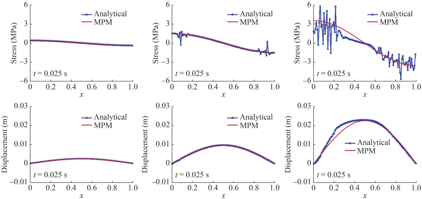Figure  16  Comparative analysis of stress and displacements in a one-dimensional vibrating bar at several time intervals

Download: Full-Size Img

• Efficient and accurate integration strategies. The material point integration in the MPM fails to satisfy integration consistency, leading to poor accuracy. Improved integration techniques use centroid integration within the background grid (Liang et al., 2019) or multiple node integration with B-spline functions (Gan et al., 2018). However, the mapping process of stress information at integration points considerably increases computational costs, focusing MPM research on efficient and accurate integration strategies.

• Issues with pressure instability and small critical time steps. The weakly compressible MPM (Lian et al., 2011a; Li et al., 2014), which does not require tracking of free surfaces, is often used to simulate complex hydrodynamics. However, it faces challenges with critically small time steps and severe pressure oscillations, as shown in Figure 17, making adaptation to large-scale ocean flow simulations difficult.

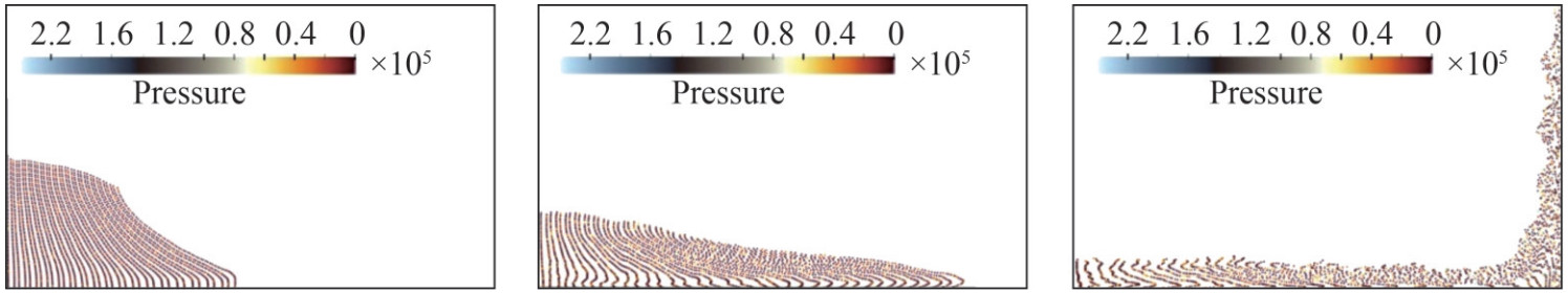Figure  17  Particle positions and pressure fields at several time instants

Download: Full-Size Img

Most of the abovementioned shortcomings result from the finite element shape functions and low-accuracy integration scheme in the MPM. Consequently, researchers have further developed other methods that allow for accurate integration on a background grid. Among these developments, the recently proposed LESCM is particularly noteworthy.

7   Lagrangian – Eulerian stabilized collocation method

The LESCM proposed by Qian et al. (2022) is an improved version of the MPM and the PIC. In this formulation, as shown in Figure 18, the SCM (Wang and Qian, 2020) is used to resolve the Navier – Stokes equations on the background Eulerian nodes. Lagrangian particles are used to describe the particle movement. The main difference between the MPM, PIC, and LESCM is that grid connection is unnecessary in the LESCM, as the SCM is truly meshfree. In addition, the integration scheme of the MPM is material point integration, whereas that of the LESCM is Gaussian integration, satisfying the integration consistency.

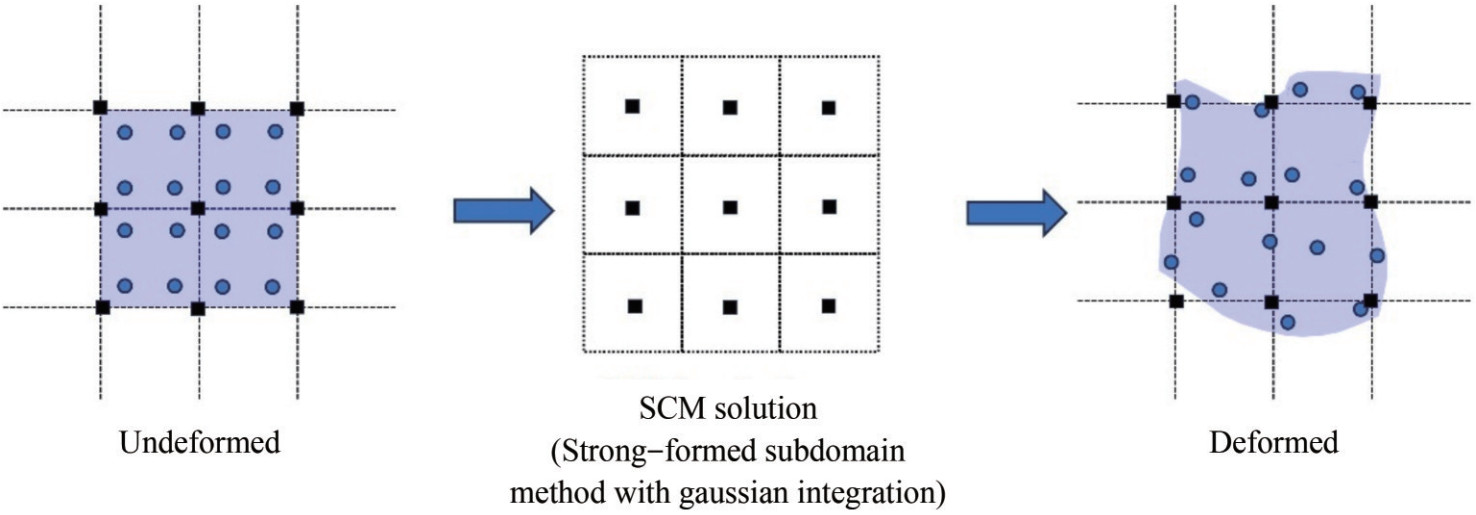Figure  18  Hybrid Lagrangian–Eulerian description in the LESCM method

Download: Full-Size Img

7.1   Brief formulation

7.1.1   Solution on the Eulerian nodes

In the SCM illustrated in Figure 18, a unique subdomain is aligned with each node in the Eulerian grid. This setup involves integrating the governing Eq. (1) over the subdo main and employing a forward difference method for temporal discretization, leading to the formulation:

where Ω_l represents the local integration subdomain for node x_l, with Ω being the problem domain of the Eulerian background grid, and Ω_l ∈ Ω or Ω_l ∩ Ω ≠ ∅. The LESCM (Qian et al., 2022), using the pressure projection technique (Chorin, 1968), divides the solution process of Eq. (36) into three distinct steps.

Step 1:

Step 2:

Step 3:

Within this framework, Eq. (38) refers to the local integration on the subdomain Γ_a^l at the solid boundary node x_l. Eq. (39), known as the integrated PPE, ensures divergence-free conditions, as indicated by:

7.1.2   Particle advection in the lagrangian framework

Post-solving the NS equations at Eulerian nodes, velocity transmission from these nodes to Lagrangian particles is crucial for particle motion and free surface tracking. The transfer scheme, depicted in Figure 19, is formulated as:

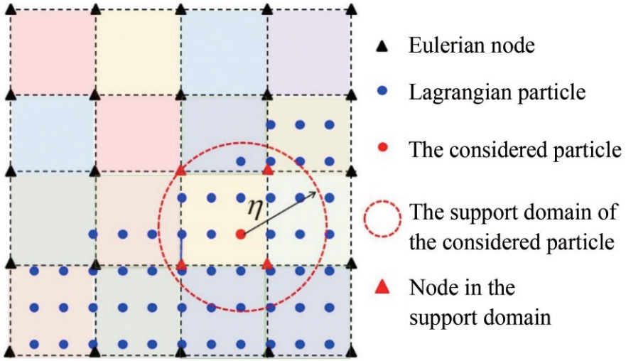Figure  19  Mapping from the Eulerian background nodes to the Lagrangian particles (This figure is reproduced from Qian et al. (2023c), Copyright (2023), with permission.)

Download: Full-Size Img

Then, we introduce a unified scheme using the velocity and acceleration mapped from the grid to calculate the particle velocity as follows (Chen et al., 2019b):

where $\overline{\boldsymbol{v}}_j^{n+1}$ is the particle velocity vector, κ = 0.03 is an empirical constant (Zhang et al., 2018b), $\hat{\boldsymbol{v}}_j^{n+1}$ is the particle velocity mapped from the grid nodal velocity (i.e., from Eq. (45)), and $\hat{\boldsymbol{v}}_j^{n+1}$ signifies the velocity vector resulting from the particle acceleration and is calculated by:

Then, Lagrangian particle positioning is updated using:

with $\hat{\boldsymbol{v}}_j$ obtained from Eq. (45). Eq. (48) is solved using the Runge–Kutta method (Kelly et al., 2015). Because explicit time integration is used for Eq. (48), the critical time step must satisfy (Qian et al., 2022):

where C_FL is an Courant number, h denotes the Eulerian node spacing, and v_maxⁿ represents the peak vⁿ value. Additionally, the direct employment of Eq. (48) might lead to uneven particle distribution, impacting simulation accuracy. Thus, the PSTs (Kelly et al., 2015) are recommended to maintain uniformity in particle distribution.

7.2   Applications in ocean engineering

LESCM was recently proposed but has already demonstrated the advantages of accuracy and conservatism and the potential for application in the fields of oceanography and coastal engineering. Currently, LESCM has the following successful applications in oceanography and coastal engineering:

• The dynamics of ocean waves, encompassing their generation, breaking, and interactions with structures.

• Water entry problems, the phenomenon of sloshing, and the interaction between fluids and solids, along with other related challenges.

• Evolutionary processes and visualization of eddy structures in ocean currents.

• The phenomenon of dam breaks.

The simulation of these phenomena and the accurate extraction of their main characteristics and energy parameters present considerable challenges to the conservation properties of numerical simulation methods. For example, as ocean waves propagate toward a coast, they change because of the coastal topography, increasing in height and breaking while continuing to spread inland. This physical process involves complex energy transfer and dissipation mechanisms. Numerical simulations with poor conservation properties can lead to the failure of many parameter predictions.

The LESCM, characterized by its dual description, conservation, and efficiency, has shown its potential in coastal hydrodynamics and offshore engineering. Initially applied to simulate straightforward scenarios such as dam breaks (Qian et al., 2023c), the LESCM has seen its applications expanded in numerous studies. In addition, Qian et al. (2023c) analyzed its conservation of mass, momentum and energy, highlighting the local and global conservation of the solutions on the background Eulerian nodes in that study. For example, the local error of the momentum solution of a dam break problem is shown in Figure 20. The magnitude of the local error is to the −14th power, which is close to the computer error. Thus, the local conservation is well guaranteed.

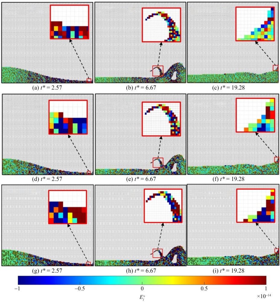Figure  20  Local error snapshots in the dam break problem at times t^∗ = 2.57, 6.67, and 19.28 (the colors on the background mesh denote the local error in the corresponding background cell): (a–c) local error of mass; (d–f) local error of linear momentum; (g–i) local error of angular momentum, here, t^∗ denote a dimensionless number related to time. (The results are reproduced from Qian et al. (2023c), with permission.)

Download: Full-Size Img

Then, the LESCM was applied to ocean wave dynamics (Qian et al., 2023b) numerical wave tank is constructed by the LESCM, and because of its good conservation and high efficiency, the LESCM obtained higher accuracy and stability than the considered methods while using a smaller resolution of particles or mesh. The local conservation, which is shown in Figure 21, was also validated in the constructed numerical wave tank. In addition, the LESCM can evaluate the interaction between structures and ocean waves, and a typical benchmark is shown in Figure 22 and Figure 23. In many cases, structures in the ocean can be modeled as rigid bodies, resulting in a fluid−rigid body interaction model. Qian et al. (2022) constructed a computational model for fluid−rigid body interactions based on the LESCM framework, enabling the LESCM to solve the problems of oceanic floats, structure entry, wall-impacting currents, etc.

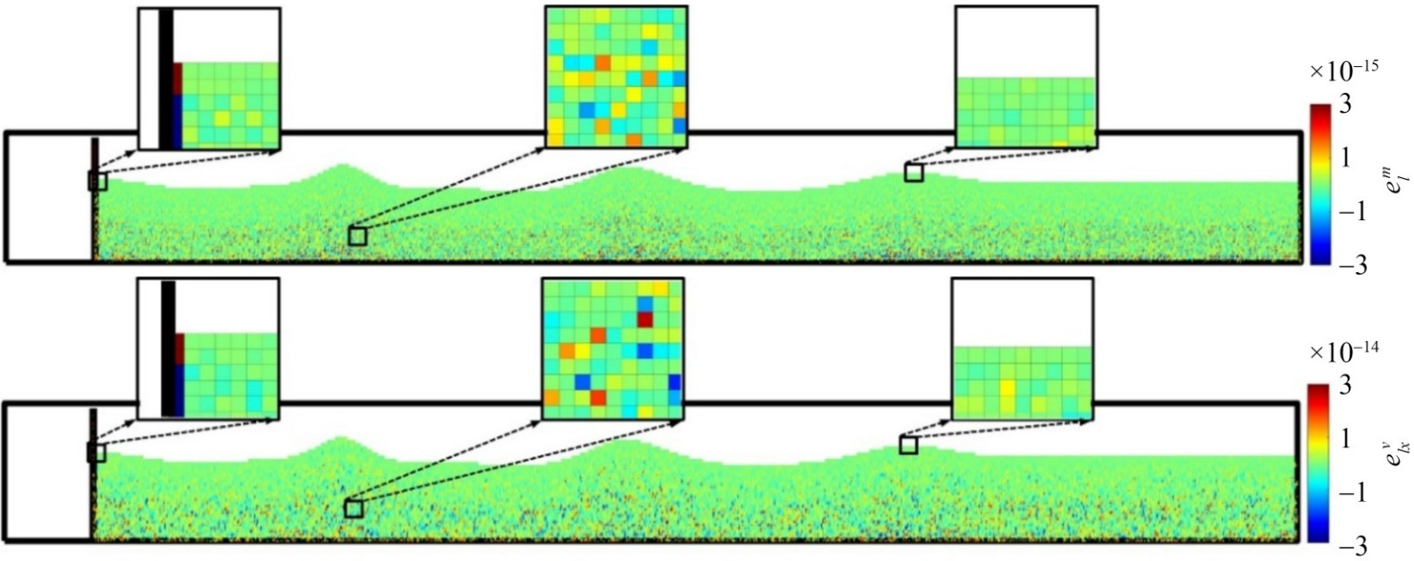Figure  21  Local error snapshots of the mass and momentum for a water wave simulation. (The results are reproduced from Qian et al. (2023b), with permission.)

Download: Full-Size Img

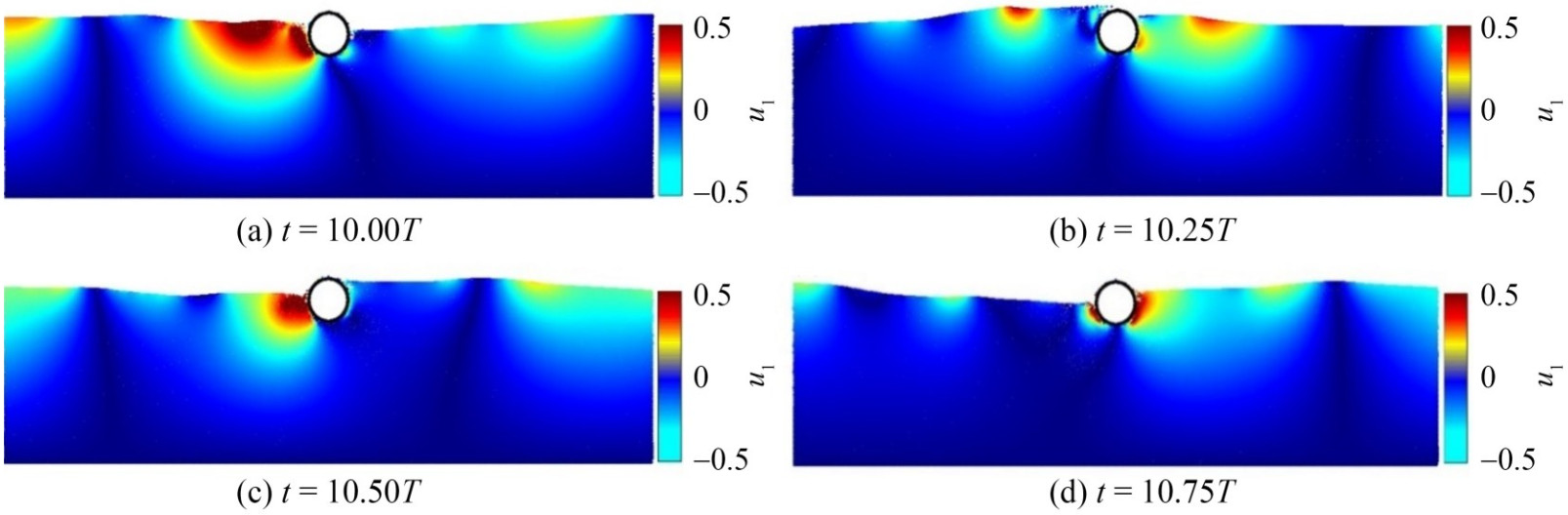Figure  22  Snapshots of the flow field of the LESCM numerical results: (a) t = 10.00T; (b) t = 10.25T; (c) t = 10.50T; and (d) t = 10.75T. (The results are reproduced from Qian et al. (2023b), with permission.)

Download: Full-Size Img

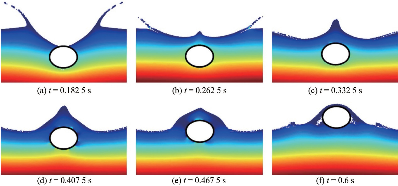Figure  23  Simulation result of the water entry of a half-buoyant circular cylinder at various times: (a) t = 0.182 5 s, (b) t = 0.262 5 s, (c) t = 0.332 5 s, (d) t = 0.407 5 s, (e) t = 0.467 5 s, (f) t = 0.6 s. (The results are reproduced from Qian et al. (2022), with permission.)

Download: Full-Size Img

Because flow visualization is another crucial subject in complicated ocean flows, the technique of extracting Lagrangian coherent structures (LCSs) is incorporated into the LESCM framework (Qian et al., 2023a). In this study, the efficiency of constructing LCSs is extremely high because the Lagrangian-type trajectories of particles are explicitly recorded in the original LESCM framework. In addition, the unphysical deformation obtained from the PST (Sun et al., 2016; Zhang et al., 2021) is avoided because the fluid deformation is computed by the fixed Eulerian nodes, not by fluid particles that have used the PST technique, enabling a reliable result of extracting LCSs. Figure 24 shows a visualization comparison between the LCS technique based on the LESCM and the traditional vortex identification technique (i.e., vorticity, the Q-criterion, and the Δ-criterion). Other methods can identify the vortex in ocean flows; however, the LCS technique provides a clear picture of the relationship between vortex structures in temporal and spatial dimensions.

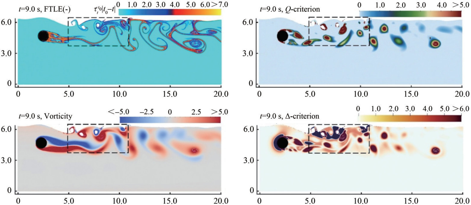Figure  24  Flow past a circular cylinder with free surfaces with Re = 200, Fr = 1.0, and h/d = 1.0: comparisons of FTLE(−), vorticity, the Q-criterion, and the ∆-criterion at t = 10 s. (The results are reproduced from Qian et al. (2023a), with permission.)

Download: Full-Size Img

7.3   Current merits and shortcomings

The LESCM is a novel hybrid Eulerian − Lagrangian method that has the following advantages:

• Truly meshfree property. The MPM and PIC methods are based on Eulerian background grids for solving the governing equations, whereas the LESCM does not require any relationship of mesh connectivity, solves the governing equations directly at the background points, and uses Lagrangian particles to describe the material motion and deformation. Therefore, LESCM is a truly mesh-free method based on the hybrid Lagrangian–Eulerian description.

• Local and global conservation. Because the SCM (Wang and Qian, 2020) is a subdomain method that can preserve local and global conservation during the solution process of the Navier – Stokes equations, local and global conservation is also guaranteed by the LESCM.

• Good stability. In the traditional MPM, stress discontinuity leads to the instability problem. In the LESCM, a high-order continuous RK is used as the shape function and the interpolation function, which stabilizes the solution and mapping process.

Given the above advantages, the LESCM has a good potential for development, particularly in high-accuracy numerical simulations of ocean flow. However, because of its relatively short development time, the following problems still exist:

• High memory requirement. The LESCM, similar to the MPM and PIC, uses a hybrid description and needs to record various information about Eulerian background points and Lagrangian particles simultaneously, resulting in a large memory requirement.

• Lack of parallelization technology. The effective resolution of large-scale ocean flow often requires parallel computing techniques, as serial methods relying on a single CPU core may prove inadequate. Regrettably, no CPU- or GPU-based parallelization approach has been devised for the LESCM, thereby constraining its applicability in addressing ocean flow challenges.

• Theoretical challenges in 3D FSI applications. Specifically, for the 3D FSI problem, the LESCM lacks a well-established and mature solution scheme. This deficiency primarily stems from the complexity of achieving efficient and highly accurate integration within the local domain, coupled with the difficult task of devising robust FSI algorithms within a three-dimensional environment.

8   Conclusions

This paper begins by reviewing the advantages and disadvantages of numerical methods based on the Lagrangian and Eulerian descriptions, then discusses the fusion of these two descriptions in the coupled description. Subsequently, it comprehensively reviews the development, implementation, and applications of various numerical methods based on the coupled description in the field of ocean engineering.

Specifically, in the ALE method, represented by the ALE-FEM, the paper discusses the implementation process of the ALE method and its research progress in areas such as tsunami simulations and wave dynamics. It also reviews open-source codes and software developed on the basis of the ALE method, briefly introducing their main functions. Following this review, the earliest hybrid Lagrangian – Eulerian particle method, namely the PIC method, is revisited. We explain its discrete process based on the hybrid description, the mapping technique between particles and the grid, and the solution process for the incompressible Navier–Stokes equations. In terms of applications in ocean engineering, the paper focuses on the research progress of PIC in wave dynamics, interactions between ocean currents and coastal structures, interactions between ocean flows and floating structures, and multiphase flows in the marine environment while also summarizing its advantages and disadvantages. In the overview of the MPM, the paper first revisits its relationship with the PIC method and its main implementation process, highlighting its advantages in simulating extreme processes (shocks, collisions, etc.). Grounded in ocean engineering, this section summarizes MPM research progress in ocean flow and structure interaction problems, detailing the application of partitioned and unified coupling technologies in solving flow–structure interaction problems with the MPM, as well as its research progress in high-accuracy numerical simulations of multiphase flows. Lastly, the paper reviews the development of the recently developed Lagrangian – Eulerian SCM (LESCM), based on a hybrid description but without the need for element connectivity on the background grid. Instead, it directly solves governing equations on background points using a meshfree collocation method, making the LESCM a purely meshfree method based on the hybrid description. Because of the introduction of local integration, this method also gains the advantages of the finite volume method, ensuring local conservation. The paper reviews the progress made by this method in fluid – structure interactions, ocean waves, and ocean flow visualization, discussing its strengths, weaknesses, and potential future development directions.

Overall, numerical methods based on the hybrid Lagrangian–Eulerian description hold great potential for many problems in engineering and science. Compared to traditional mesh-based numerical models, they excel in handling large deformations and tracking free surfaces, moving interfaces, and deformable boundaries. Compared to traditional particle-based numerical models, they eliminate the need for neighborhood particle searches, considerably improving computational efficiency. They also avoid stretch instability, enhancing the accuracy and stability of numerical solutions. These methods are poised for rapid development in future high-accuracy numerical simulations of ocean flows.