1   Introduction

In recent years, the role of AUVs has significantly increased to perform undersea exploration missions. The potential of AUVs has been substantially increased due to the advancements in various technologies. These technologies include, but are not limited to, advanced sensor capabilities, AI-driven autonomy, efficient hydrodynamic design, improved energy storage solutions, robust communication systems, smart navigation and localization techniques, and advanced materials technology (Ahmed, et al., 2023a; Karimi & Lu, 2021; Mohsan et al., 2022; Zhao et al., 2022).

The AUVs' multifaceted attributes, including access to challenging undersea terrains, independent navigation, prolonged operational endurance, and efficient data collection, make them as essential tools to perform underwater tasks for commercial as well as military applications (Sun et al., 2020; Zhang et al., 2018). The AUVs have made substantial contributions to areas like oceanography, seafloor mapping, environmental monitoring, oil & gas exploration and reconnaissance missions. The performance efficiency and cost-effectiveness of AUVs in conducting underwater surveys have streamlined scientific investigations, resource identification, and environmental assessments (Li et al., 2023b).

The underwater vehicles should be hydrodynamically stable, efficient and capable of performing the six-degrees of freedom maneuvers in harsh and unpredictable undersea environment. To achieve better hydrodynamic design of an AUV, the drag polar curve provides important and comprehensive understanding of the intricate balance between lift and drag forces observed by an AUV while maneuvering underwater at different angles of attack and varying speeds (Javanmard, et al., 2020b). Improved lift-to-drag ratios enhance energy efficiency and extend operational range of an AUV and the drag polar curve provides the optimal operating points where the lift is maximized and the drag is minimized. The curve also provide insights in evaluating AUVs' stability and maneuverability by examining the changes in lift and drag at various angles of attack and speeds (Guerrero et al., 2012). To model the thrust requirements of an AUV, it is essential to estimate the axial drag and for an efficient hydrodynamic design, the axial drag is to be kept as minimum as possible. Accordingly, the drag curve also provides valuable data for modeling the thrust and power requirements.

In addition to various other factors, the impact of bubbles and cavities in the water have significant implications on the hydrodynamic design of AUVs. Bubbles can introduce additional drag to the AUV, while cavitation, particularly at higher speeds, can detrimentally affect propulsion efficiency and overall hydrodynamic performance of an AUV. Therefore, to investigate dynamics of oscillating bubbles such as cavitation bubbles, underwater explosion bubbles, and air bubbles, a novel theory to model complex multi-cycle bubble dynamics, providing new physical insight into inter-bubble energy transfer and coupling of bubble-induced pressure waves, have been recently introduced (Zhang et al., 2023a).

Overall, accurate prediction of flow characteristics such as velocity distribution, drag forces, added mass and lift forces, is essential for enhancing the hydrodynamic efficiency and maneuverability of AUVs (Ahmed, et al., 2023c; Javanmard, 2020a; Randeni et al., 2022).

Computational Fluid Dynamics (CFD) tools are increasingly become important to study the fluid flow dynamics around the AUVs for optimizing their hydrodynamic design, maneuverability, and overall performance (Ahmed, et al., 2023b). CFD application for underwater fluid flow simulations are not only limited to the study of flow region from laminar to turbulent flow transitions but these are recently extended to simulate the complex fluid dynamics phenomena, such as supercavitation in high-speed underwater vehicles. For instance, in (Huang et al., 2022) researchers employed CFD to investigate the behavior of compressible supercavitation flows around supersonic supercavitating projectiles. The study focused on understanding the flow field during the deceleration phase, where the projectile transitions from supersonic to subsonic speeds.

CFD simulations involve solving the Reynolds-Averaged Navier-Stokes Equations (RANSE), derived from the Navier-Stokes equations by incorporating Reynolds averaging techniques, to analyse the incompressible, Newtonian fluid flow around the underwater vehicles (Javanmard, et al., 2020b). To solve the fluid flow Navier-Stokes governing equations through CFD techniques to simulate the flow around AUVs is a common practice and can be achieved using various commercially available CFD tools including, STARCCM+, ANSYS Fluent, CFX and others (Gao et al., 2022; Go & Ahn, 2019; Javanmard, et al., 2020b; Zhang et al., 2010; Zhang et al., 2022). Besides, Solidworks Flow Simulation (SWFS) is also considered one of the commonly used CFD tool to perform fluid flow analysis for various engineering applications (Korres et al., 2019; Matsson, 2023; Mohanty et al., 2023; Rodriguez et al., 2019; Zhang et al., 2023c). However, despite having vast availability of the CFD tools, it is still challenging to perform the CFD simulations to achieve the accurate results at minimal computational cost and time. The researchers continuously look for trade off between the accuracy, computational resources, user friendly meshing techniques, boundary layer treatments and improved approaches to turbulence modeling provided by these CFD tools.

To simulate unsteady underwater turbulent flows for higher Reynolds number using RANSE requires averaging the fluid flow governing equations over the time to separate the mean flow from the fluctuating turbulent flow. The averaging process introduces additional terms called Reynolds stresses, which need to be modelled in order to close the system of equations. Usually, two-equation turbulence models k − ϵ and k − ω models are used for closure of the Reynolds stresses by solving additional transport equations for the turbulent kinetic energy (k) and dissipation rate (ϵ or ω). In RANS simulations, the equations for the mean flow variables (velocity, pressure, etc.) and the two turbulence model equations (k and ϵ or ω) are solved simultaneously to obtain a solution that represents the averaged flow properties and the turbulence characteristics (Jagadeesh et al., 2009; Kadivar and Javadpour, 2021; Menter, 1994). However, to effectively model the turbulent flow is a complex and challenging task. Consequently, a significant focus of researchers remained on effectively modeling turbulence phenomena while solving RANSE through CFD techniques (Guo et al., 2023; Jagadeesh & Murali, 2005; Phillips et al., 2007; Vardhan & Sztipanovits, 2023; Wang et al., 2023). For instance, Lidtke et al. (2017) used k_L − k_T − ω RANS model by Walters and Cokkjat (2008) to model the transition flow to observe more realistic hydrodynamic performance of an underwater glider, particularly at the initial design stage.

Additionally, mesh refinement techniques and solution convergence analysis are also considered important factors in CFD simulations as these directly influence the accuracy and computational efficiency of the simulations (Javanmard, 2020a; Li et al., 2023a; Rizk et al., 2023; Xiang et al., 2020).

In this paper CFD-based hydrodynamic lift and drag estimations of a newly designed torpedo-shaped flight-style AUV with bow-wings maneuvering at different angles of attack and speed are presented. Accordingly, in the present study the RANSE closure is achieved using modified k − ϵ model to capture the turbulent flows and Two-Scale Wall Function (2-SWF) approach is employed for the wall treatment. Moreover, unique mesh refinement and solution-adaptive features offered in SWFS environment have been used which allows the mesh to dynamically evolve during the simulations while adapting to the flow characteristics and capturing boundary layer phenomena more accurately (Wallace, 2019). Simulated results, particularly for axial drag, have been compared with experimental findings obtained through free running underwater experiments of flight-style AUV. The main contribution presented in this article are three-fold and summarized as follows:

• CFD-based hydrodynamic design analysis of novel bow-wings AUV: Computed drag and lift forces for different angles of attack and speed of novel flight-style AUV. Insights from drag polar curve for AUV with and without bow-wings have been provided.

• SWFS capabilities to simulate the fluid flow around AUV: The RANSE closure is achieved by employing the modified k − ϵ model. For boundary layer treatment 2-SWF approach is used. Further, mesh refinement and solution-adaptive meshing features of SWFS have also been discussed in detail.

• Experimental validations: Simulated results for axial drag have been compared with free running underwater AUV maneuvering test results.

The paper is structured as follows: After the introduction, Section 2 presents the features and characteristics of the novel flight-style AUV. In Section 3, simulated results for lift and drag using CFD methods are provided. Subsequently, insights from the drag polar and axial drag are discussed in Section 4. Section 5 includes experimental validations of simulated axial drag, and it also provides insights into the relationship between the AUV thrust and drag. Finally, the study is concluded in Section 6.

2   Flight-style AUV: features and characteristics

The AUV, shown in Figure 1, has been designed and developed by the Lab of Advanced Robotic Marine Systems (ARMs), School of Naval Architecture and Ocean Engineering (SNAOE), Huazhong University of Science and Technology (HUST), Wuhan, China (Zhang et al., 2023b). The AUV is featured with a unique modular design equipped with removable bow-wings and fins subject to the application requirements. This study refers AUVs with bow-wings and without bow-wings as AUV₁ and AUV₂, respectively (see Figure 2).

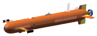Figure  1  Torpedo-Shaped Flight-Style AUV with bow-wings

Download: Full-Size Img

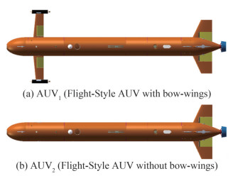Figure  2  Reversible configurations of Flight-Style AUV

Download: Full-Size Img

The flight-style AUV with bow-wings is mainly designed and developed to perform the complex undersea cable detection and tracking operation in harsh sea environment. Therefore, it requires efficient and stable hydrodynamic design having better lift-to-drag ratio. The provision of bow-wings has dual purpose: one is to mount the electromagnetic arrays on each bow wing and the other is to provide the improved and efficient hydrodynamic performance of the AUV. Hence, the design optimization of the bow-wings has been focused to fulfil the functional requirements as well as to achieve improved hydrodynamic performance by generating maximum lift with minimal drag.

Moreover, following the fixed-wings aircraft design, the AUV is provided with fixed-wings as well as moving control planes (fins) at both stern and bow ends of the AUV. Both fixed-wings and moving fins follow the NACA 0010 profile. The length (l) and diameter (d) of the AUV are 2.71 m and 0.24 m respectively. Unlike the traditional torpedo-shaped AUV, the flight-style AUV has relatively larger length-to-diameter ratio (l/d is 11.3). The dry weight of the AUV is approximately 85 kilograms. 3D CAD models of the AUV hull, wings, fins and other sub-assemblies have been generated using Solidworks CAD software. Exploded view of the flight-style AUV indicating the main sections and sub-sections is shown in Figure 3.

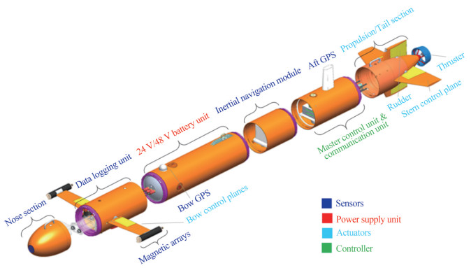Figure  3  Exploded view of Flight-Style AUV

Download: Full-Size Img

The flow characteristics of the AUV with bow-wings encompass hydrodynamic efficiency, lift and drag performance, stability, maneuverability, and overall fluid dynamics behavior. These aspects are shaped by the AUV's form, wing design, control surfaces, and hydrodynamic attributes. The bow-wings introduce unique flow interactions that impact lift generation, drag reduction, and overall underwater performance. Accordingly, in this study drag curves for both the configurations of AUV that is with and without bow-wings have been investigated.

3   CFD simulations

The continuity and momentum equations are given in equations 1 and 2 respectively (Anderson & Wendt, 1995; Yu et al., 2023).

where, ρ is the fluid density, p is the pressure term, ν is the dynamic viscosity, u_i is the flow velocity components and $ \rho \overline{u_i^{\prime} u_j^{\prime}}$ is the Reynolds stress tensor which characterizes the turbulent behaviour of the fluid flow and captures the correlations between the fluctuating velocities u_i and u_j within the flow field.

The RASNE closure in SWFS achieved by utilizing transport equations for turbulent kinetic energy and its dissipation rate, employing the modified k − ϵ model. The classical two equation k − ϵ turbulence model (Wilcox, 1994) is modified by applying empirical adjustments to capture the variety of turbulent flows such as rotational and shear flows.

The modified k − ϵ turbulence model with damping functions (Lam & Bremhorst, 1981; Sobachkin & Dumnov, 2013) characterizes the behavior of laminar, turbulent, and transitional flows in the governing equations of the conservation laws.

where, C_μ = 0.09, C_ϵ1 = 1.44, C_ϵ2 = 1.92, σ_k=1, σ_ϵ = 1.3, σ_B = 0.9, C_B =1 if P_B > 0, C_B = 0 if P_B < 0.

Further, turbulent viscosity μ_t and Lam & Bremhorst's (Lam & Bremhorst, 1981) damping function (f_μ, f₁ & f₂) are defined in equations 6 and 7, respectively.

where, $ R_y=\frac{\rho \sqrt{k} y}{\mu}, R_t=\frac{\rho k^2}{\mu \epsilon}$ and y is the distance to the wall from the point.

In case the damping functions f_μ, f₁ and f₂ are equal to 1, the modified k − ϵ models turns to be the original k − ϵ (Lam & Bremhorst, 1981; Sobachkin & Dumnov, 2013).

3.1   Boundary layer treatment

SWFS directly utilizes the native CAD format as the primary source of geometry information and seamlessly combines with 3D CFD modeling even when the mesh resolution is insufficient for a complete 3D simulation (Sobachkin & Dumnov, 2013). The non-body-fitted Cartesian meshes are considered optimal for handling native CAD data serving as the fundamental basis for the CAD/CFD integration. However, the main challenge with Cartesian immersed-body meshes is the resolution of boundary layers on 'coarse meshes'. Accordingly, a unique 2-SWF approach is employed in SWFS, combining with its Cartesian mesh technology for CAD/CFD integration. When the mesh at the solid-fluid interface (near-wall cells) is too coarse for accurate Navier-Stokes equation solving in the high-gradient boundary layer, the 2-SWF approach is used for wall treatment. The process for coupling boundary layer is delineated as follows (Sobachkin & Dumnov, 2013):

• If the number of cells near the boundary layer is insufficient, a thin boundary layer treatment is employed.

• If the number of cells across the boundary layer exceeds the necessary amount for accurately resolving the boundary layer, a thick boundary layer approach is utilized.

• A combination of both thin and thick boundary layer treatments can also be applied, depending on the specific problem requirements.

Utilizing the CAD/CFD integaration capabilities of SWFS, the fluid flow around the flight-style AUV, CAD modelled in Solidworks, has been simulated.

3.2   Meshing techniques

Both global and local meshing techniques have been employed to discretize the computational domain for fluid flow simulations around the AUV, as depicted in Figure 4. The global mesh feature in SWFS enables users to define the initial mesh with refinement levels ranging from 1 to 7. It can be seen in Figure 4 that the cell size decreases when the mesh progresses from the outer boundary of the domain to the surface of the model.

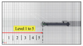Figure  4  Global mesh refinement to level 5 and higher mesh density around the AUV

Download: Full-Size Img

To accurately capture high-gradient flows or flow patterns passing through complex geometries, local meshing techniques are applied. These techniques enable precise modeling of boundary layers, recirculation zones, and localized flow behavior.

Additionally, solution-adaptive meshing feature of SWFS allows the users to refine the mesh dynamically during the run-time simulations.

The software splits the mesh cells in the high-gradient flow regions and merge the cells in the low-gradient flow regions which ensures better accuracy during the calculation. The requisite modification to the initial state of the mesh is achieved by selecting the level of refinement from the 'calculation control option' dialogue window. The refinement level indicates that how many times the initial mesh cells can be divided to achieve the solution-adaptive refinement criteria. Simply each cell is segmented into smaller successor cells.

To achieve optimal solution with minimal computational effort, SWFS meshing techniques are systematically evaluated for various settings. Accordingly, following two different case studies have been conducted:

Case Study (1): The study includes three sets of flow simulations having distinct mesh configurations: coarse, medium and fine. The size of computational domain was automatically determined by the software based on the size of the AUV model. To evaluate the impact on computational results, mesh refinement techniques including global refinement, local refinement, and auto-meshing have been applied.

Case Study (2): The study includes three different sets of flow simulations having different domain sizes with fixed global mesh refinement level to 3. Additionally, flow simulation were also performed with global mesh refinement level to 5.

Simulation parameters configuration for both the case studies are presented in Tables 1 and 2 respectively. In both the case studies, the axial drag has been computed for the AUV speed of 1kn. The convergence criteria was set to achieve the target value of 10⁻⁶, ensuring the solution reached a steady state for velocity and drag. Computational meshed domain is shown in Figure 5.

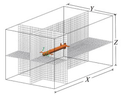Figure  5  Computational domain

Download: Full-Size Img

3.3   Case study (1): findings and analysis

The effect of mesh refinement on computational results is investigated in this study and three sets of simulations have been performed. The input and output parameters are presented in Table 1 and 3 respectively. The first set of simulation (Figure 6a) is performed on coarse mesh with global mesh level of 3. Subsequently, the mesh is refined from coarse to medium and global mesh refinement level increased to 5 during the second set of simulations (Figure 6b). In the third set of simulation (Figure 6c), similar settings as the medium mesh have been employed, however, an auto-mesh refinement option is activated during the simulation run at iteration 47. A higher global mesh level necessitates flow calculations across the entire computational domain, consequently leading to an increased computational cost. Alternately, the auto-meshing technique improves computational efficiency by dynamically refining the mesh, directing more cells to regions with complex flow, and reducing cell density in areas characterized by uniform flow. Subsequent to the iteration 47, rapid convergence of variables (velocity and drag) have been observed. Figure 7 shows the linear relationship between mesh refinement and the convergence of velocity and drag in all three simulation sets. Once values reach a steady state, the solver halts further computations. The use of wall functions, compared to Y+ methods, reduces the need for extremely fine meshes near solid surfaces or within boundary layers. Thus, 2-SWF offers flexibility in mesh coarseness to capture the near-wall flow behavior while reducing sensitivity to mesh refinement near solid surfaces.

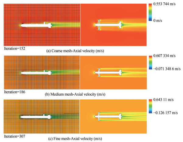Figure  6  Velocity contours for different mesh configurations

Download: Full-Size Img

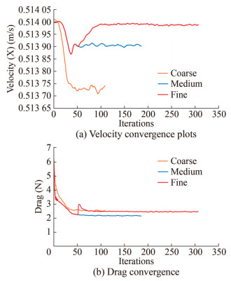Figure  7  Velocity and drag convergence plots

Download: Full-Size Img

3.4   Case study (2): findings and analysis

In this case study, three different sizes of computational domains A, B, and C are defined such that C > B > A. The global domain mesh refinement level was set to 3 for all three domain sizes. It ensures consistent level of mesh detail throughout the simulations and enhances the accuracy of the results by capturing the flow features and gradients. Additionally, the auto-meshing refinement has been activated at iteration number 47. Additional results are also obtained using computational domain C with domain mesh refinement level 5, and auto-meshing feature activated at iteration number 52. The simulated results are presented in Table 4.

Figure 8 depicts the mesh density and velocity contours for the three types of domain sizes. These visual representations are useful in comprehending the distribution of mesh and flow patterns within the domains. The plots in Figure 9 offer insights into the behaviour and convergence trends of these flow parameters which help to analyse the impact of domain size and mesh refinement on the simulation results. However, appropriate selection of domain size and mesh refinement levels are required to trade-off between accuracy and computational cost and time.

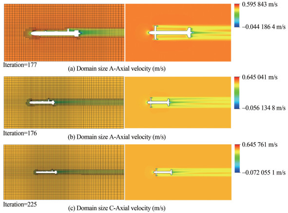Figure  8  Velocity contours for different domain sizes

Download: Full-Size Img

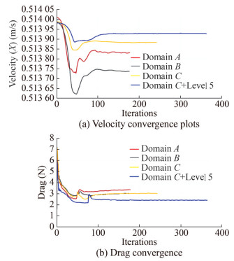Figure  9  Velocity and drag convergence plots

Download: Full-Size Img

3.5   A quantitative assessment: standard deviation (σ) and coefficient of variation (CV) calculations

To quantify the spread or variability of the computed results of axial drag of the AUV in both the case studies, standard deviation calculations have been performed using equation 8. A higher standard deviation indicates a greater dispersion or variability in the computed results, while a lower standard deviation suggests more consistency or similarity among the computed data.

where, σ is the standard deviation of sample data, x is individual data in the sample, ν is the mean of the data sample and N is the total number of data points in the sample.

To further examine the standard deviation (σ) as a percentage, coefficient of variation (CV) has been calculated using the equation 9.

The computed results for both the studies in terms of (σ) and CV are presented in Table 5.

Based on the results summarized in Table 5, it can be inferred that suitable mesh densities can be selected for CFD simulations using SWFS tool. Since, in SWFS, wall function are used for boundary layer treatment in a computational domain, therefore, increasing the mesh density near the walls of the AUV may not yield significant improvements as the same is evident from the findings elaborated above. However, it is essential to strike a balance between computational cost and accuracy. From the analyses, it can be deduced that for the streamlined shapes such as torpedo-shaped AUV, the domain size generated by SWFS considering the size of the model geometry is considered sufficient to simulate the fluid flow past over the object, unless specific far field boundary treatments are required. Moreover, by optimizing the mesh settings and employing a mesh refinement level of 3 ‒ 5 with default computational meshed domain, it is possible to conduct fluid flow simulations around the AUV with acceptable accuracy. These results can be achieved with minimal computational efforts in SWFS environment as compared to traditional CFD tools, which typically require extensive user expertise in creating the computational domain, meshing the domain, boundary layer treatments specially near the wall and careful consideration of Y+ resolution. Hence, CFD tools like SWFS offer a favourable alternative, allowing for efficient simulations of fluid flow around the AUV with acceptable accuracy while minimizing the effort required for domain setup and meshing, particularly in comparison to other conventional CFD approaches.

Finally, based on the findings from the above two case studies, series of simulations have been conducted to estimate the drag and lift forces at different speeds and angles of attack for both the configurations of AUV.

4   Drag polar curve

To achieve hydrodynamically efficient design of an AUV, it is required to achieve higher lift with lesser drag as much as possible. Accordingly, drag polar curve offer insights into hydrodynamic performance of AUV and considered useful to evaluate the efficiency, stability, and maneuverability of AUV under varying conditions.

An example of a drag polar curve of a symmetrical wing is illustrated in Figure 10. The figure shows the relationship between the drag coefficient (C_D) and the lift coefficient (C_L). Where, C_D0 represents the minimum drag coefficient (C_Dmin) and coincides with the extremum of the parabolic-shaped drag polar curve. At this point, C_L is equal to 0, as illustrated in Figure 10.

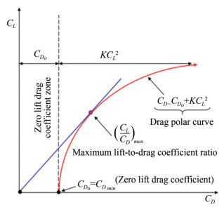Figure  10  Example of drag polar curve for a symmetrical wing (Guerrero et al., 2012)

Download: Full-Size Img

The tangent line originating from the origin of coordinates identifies the maximum lift-to-drag ratio (C_L/C_D)_max. The intersection of the drag polar curve with the C_D axis corresponds to C_D0, gives minimum drag value. The area between the polar curve C_D0 + KC_L² and C_D0 represents the induced drag (C_Di) which is proportional to C_L². Each point on the drag polar curve corresponds to a different angle of attack of the wing. For symmetrical wings, the total drag can be expressed as C_D = C_D0 + KC_L² (Guerrero et al., 2012).

Considering the top/bottom and port/starboard shape symmetry of the flight-style AUV, the drag polar curve is taken as reference to comprehend and interpret the computed (C_L/C_D) values for both the configurations of flight-style AUV (see Figure 10).

To establish the drag polar curve for flight-style AUV, a series of simulations have been performed and estimated the drag and lift forces for angles of attack (−3°, 0°, 3°, 6°, 9° and 12°) and different speeds of AUV ranging from 1‒6 knots. The simulated results for drag and lift forces for both configurations of the flight-style AUV (AUV₁ & AUV₂) at different angles of attack and flow speeds are presented in Table 6 and Table 7 respectively. Figure 11a–11f shows the change in lift and drag with angle of attack and speeds of AUV. Additionally, Figure 12a–12b shows velocity contours of AUV cruising underwater at the speed of 3 knots at an angle of attack −3° and +6°, respectively.

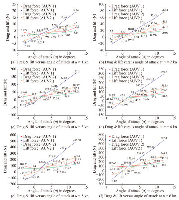Figure  11  Drag and lift forces observed by AUV maneuvering underwater at different angles of attack and varying speeds

Download: Full-Size Img

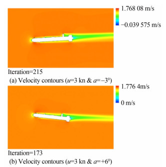Figure  12  Velocity contours of AUV at u=3 kn, α=−3⁰ & 6⁰

Download: Full-Size Img

The maximum lift-to-drag ratio represents the optimal balance between the lift and drag forces such that the AUV achieves the maximum lift for the minimum drag. A higher lift-to-drag (L/D) ratio of an AUV indicates better hydrodynamic performance. Accordingly, from the results tabulated in Tables 6 and 7 and demonstrated in Figure 12, it can be seen that AUV₁ showed higher lift-to-drag ratios compared to AUV₂ thereby, demonstrating superior hydrodynamic efficiency and improved performance. In fact, the addition of bow-wings played significant role in enhancing the hydrodynamic performance of AUV₁ by enabling efficient lift generation with minimum addition of drag and thus resulted in increased overall performance of AUV in terms of speed, range, and endurance.

The computed results of lift coefficient C_L, drag coefficient C_D and corresponding lift-to-drag coefficient (C_L/C_D) ratios are presented in Table 8. The computed values are used to generate the drag polar curves for AUV₁ & AUV₂ as shown in Figure 13.

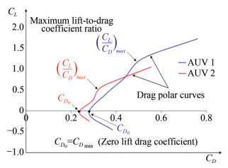Figure  13  Drag polar curve of AUV₁ and AUV₂

Download: Full-Size Img

5   Experimental validations: axial drag

5.1   AUV thrust and drag relationship

The drag observed by the AUV while maneuvering underwater corresponds to the 'reduced thrust' produced by the propeller. When the propeller is mounted at aft of the AUV, the performance of the propeller is reduced and denoted by the thrust reduction factor t. The value of t ranges between 0.25‒0.4 (Min et al., 2020; Pivano, 2008). The relationship between the thrust and drag are as follows (EV, 1989):

where, T is propeller thrust, ρ is density of water, n is revolutions per second, d is propeller diameter, R_T is hull resistance/drag, C_DT is drag coefficient, K_T is thrust coefficient, S is surface area of the AUV hull and U is the speed of AUV.

The propeller characteristics can be defined using a non-dimensional variable J, which is known as 'advance ratio' and can be computed as $ J=\frac{U}{n d}$. The thrust coefficient C_DT can be estimated by re-arranging the terms in equation 10 and given as follows.

5.2   Propeller thrust–Mooring thrust test

To meet the thrust and propulsion requirements of the flight-style AUV, a thruster named 'Whale 1 214' as shown in Figure 14, has been designed and developed by an inland manufacturing facility. It is a compact and high-efficiency deep-sea thruster with a specialized shrouded propeller. With its maximum diameter of only 140 mm, it manages to achieve an impressive performance within a small form factor. Power rating of the electric motor is 450 W.

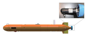Figure  14  Thruster 'Whale 1 214'

Download: Full-Size Img

The thruster is capable to generate maximum thrust of 14.8 kg to propel AUV through the water. Additionally, it has a rated mooring thrust of 12.5 kg, indicating its ability to provide consistent and stable thrust during stationary operations, such as holding a specific position or maintaining a steady heading as shown in Figure 15. The thruster is capable to operate reliably in challenging underwater environments at a depth of up to 6 000 m.

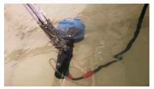Figure  15  Mooring thrust and fatigue test

Download: Full-Size Img

The characteristics of a screw propeller encompass several non-dimensional coefficients, which involve factors like advance velocity, revolutions, propeller diameter, and water density (Newman, 2018). These non-dimensional coefficients are derived from the Propeller Open Water (POW) test results. From these coefficients the thrust and torque at specific rotational speeds can be estimated (Lee et al., 2010). The rotational speed and thrust measured during the mooring thrust and fatigue test are presented in Table 9.

5.3   Free running underwater experiments

The free running underwater experiments of AUV were conducted in an inland lake located at Cangzhou City, Hebei Province, China as shown in Figure 16.

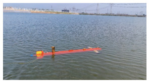Figure  16  Free running experiments of flight-style AUV

Download: Full-Size Img

Considering the mooring thrust data (Table 9) and relationship for thrust and resistance in equation 10, the axial drag observed by the AUV have been estimated during the free running underwater tests. Velocity curves for AUV speeds 2 kn, 3 kn and 4 kn and propeller rotational speed in rpm recorded during the free-running underwater tests are shown in Figure 17a and Figure 17b, respectively. The thrust reduction factor considered to be 0.4 (Min et al., 2020; Pivano, 2008).

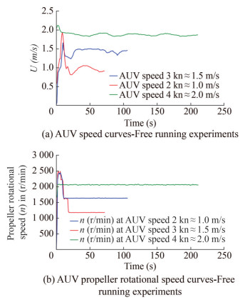Figure  17  Free running underwater experimental data-AUV speed and propeller rpm curves

Download: Full-Size Img

Figure 18 shows the actual trajectory of flight-style AUV maneuvering at 3 kn during underwater tests.

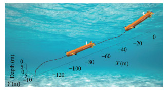Figure  18  AUV trajectory during the free running experiment

Download: Full-Size Img

The comparison between simulated and experimental results for axial drag observed by AUV₁ is shown in Figure 19. Moreover, to differentiate between both configurations of AUV with respect to the effect of bow-wings on axial drag, the results for drag observed by AUV₂ are also presented in Figure 19.

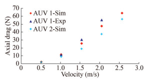Figure  19  Axial drag-Simulated and free-running underwater experimental results

Download: Full-Size Img

6   Conclusion

In this study, CFD techniques, particularly using the modified k − ϵ model and Two-Scale Wall Function (2-SWF) approach within the SWFS environment, have been employed to evaluate the hydrodynamic performance of a novel flight-style AUV equipped with bow-wings. Specifically, the horizontal bow-wings have been designed and integrated with the flight-style AUV for the dual purpose: one is to accommodate the electromagnetic arrays which are required for cable detection and tracking near the seabed and secondly to enhance the overall hydrodynamic performance of the AUV. The lift and drag have been estimated through a series of CFD simulations for two configurations of flight-style AUV: one with bow-wings and the other without bow-wings. The simulations were performed for AUV maneuvering at various angles of attack and speeds. The performance of both the configurations of flight-style AUV in simulation environment found consistent.

The drag polar curves for both the configurations of AUV have been generated using the computed lift and drag coefficients. The AUV equipped with bow-wings demonstrated improved lift and drag characteristics compared to the AUV without bow-wings. The drag polar curve highlighted a better lift-to-drag ratio for flight AUV with bow-wings as compared to the traditional torpedo-shaped AUV with wings and control surfaces only at the aft end. Overall, the findings emphasize the potential benefits of the bow-wings in enhancing the overall hydrodynamic performance of the AUV, contributing to improved stability and efficiency during underwater maneuvers, particularly to perform the specialized tasks. Additionally, simulated results for axial drag observed by the AUV maneuvering at different speeds at 0 angle of attack have also been compared with experimental results and were found in good agreement.