Unsteady RANS CFD Simulation on the Parametric Roll of Small Fishing Boat under Different Loading Conditions
https://doi.org/10.1007/s11804-024-00427-0
-
Abstract
Fishing boats have unique features that make them prone to changing loading conditions. When the boat leaves the port, the empty fish tank gradually fills up during fishing operations which may result in parametric roll (PR). This dangerous phenomenon that can lead to capsizing. The present study aims to understand better the behaviour of parametric roll in fishing boats and its relation to changing loading conditions. The study considers the effects of displacement and the GM/KM ratio on parametric roll, as well as the longitudinal flare distribution at the waterline. Two assessments to detect the parametric roll occurrence in early stage were carried out by using the level 1 assessment of parametric roll based on the Second Generation of Intact Stability criteria (SGIS) from International maritime Organisation (IMO) and the Susceptibility criteria of Parametric roll from the American Bureau of Shipping (ABS). Then, the CFD method is used to predict the amplitude of the parametric roll phenomenon. The results provide important insights to fishing vessel operators on how to manage loading conditions to maintain stability and avoid hazardous situations. By following the guidelines outlined in this study, fishing boats can operate more safely and efficiently, reducing the risk of accidents and improving the overall sustainability of the fishing industry.-
Keywords:
- Small fishing boat ·
- Parametric roll ·
- URANS-CFD ·
- KRISO Container Ship (KCS) ·
- Stability in waves
Article Highlights• The study provides a deeper understanding of parametric roll in fishing boats, a dangerous phenomenon that can lead to capsizing, and its relation to changing loading conditions.• The effects of displacement and the vertical load position (GM/ KM) on parametric roll are considered, along with the longitudinal flare distribution at the waterline.• Two assessments were used to detect the occurrence of parametric roll in the early stages, based on the Second Generation of Intact Stability criteria from IMO and the Susceptibility criteria of Parametric roll from ABS.• CFD simulations, used to predict the amplitude of parametric roll, revealed the importance of keeping the y+ value below unity to accurately model the viscous effect on parametric roll amplitudes.• The study also highlighted the role of the GM Ratio (level 1 assessment of PR on SGIS from IMO) in changing the amplitudes of parametric roll, pitch, and heave motions. -
1 Introduction
Parametric roll is one of the five stability failures that should be investigated in the design phase recommended by IMO on the Second Generation of Intact Stability (SGIS). Parametric roll occurs because of the periodic variation of the restoring roll moment. When the ship moves in waves, especially in head waves, the GM changes considerably during one encounter period. Usually, the GM is low when the wave crests at the midship and high when the wave trough at the midship. These changes trigger the roll motion gradually. When the encounter frequency is twice the roll's natural frequency, parametric resonance occurs (Park et al., 2013).
The occurrence of parametric roll can be identified early in the design spiral using the relationship between the encounter wave period (Te) and natural roll period (Tn). The phenomenon is predicted to occur where the ratio Te/Tn is close to 0.5. However, the amplitude of parametric roll should also be predicted to ensure the boat's safety, and comfort during operation. In the worst case, high roll amplitudes may lead the ship to capsize because of insufficient restoring moment.
Parametric roll studies have mostly focused on large ships, such as ONR Tumblehome surface combatant (Sadat-Hosseini et al., 2010; Liu et al., 2021) and container ships (Park et al., 2013; Yu et al., 2018; Yu et al., 2019; Zhou et al., 2016). While many researchers focused on investigating the parametric rolling of large ships, some researchers investigated fishing boats, such as Neves (2002), Ghamari et al. (2017) and Ghamari et al., (2020). Based on these publications, fishing boats can experience parametric roll in the same way as merchant ships as long as the conditions triggering parametric roll are met.
However, the length of the fishing boats mentioned in the above studies investigated large vessels, approximately 25 m in length, which is not sufficiently small to represent a large portion of today's fishing boat fleet. There are considerable differences in the seakeeping behaviour between large and small vessels. Subject to the same wave at sea, the response of small boats tends to be higher than large vessels, making them uncomfortable. Moreover, to the best of the authors' knowledge, there are no existing studies investigating the parametric roll of small fishing boats by using fully nonlinear unsteady RANS simulations, especially in different loading conditions. The present paper models a typical five-metre Indonesian fishing boat to investigate its parametric roll behaviour as a case study.
The Republic of Indonesia's territorial waters span a greater area than the country's landmass. The natural resources from this area, especially the fish resource, should be well utilised for the welfare of the Indonesian people. Thus, research about the fishing boat has become essential to ensure fishing activities in Indonesia are safe. Many fishing boats in Indonesia are built in small sizes.
Small fishing boats are the most prone to accidents compared to the large ones. Moreover, Iqbal et al. (2023) showed that the operability of small fishing boats is not high, around 60% ‒ 70%, due to several strict seakeeping criteria, such as limits on RMS roll amplitudes. Due to the small typical boat size, the roll natural period of the small fishing boat is relatively low and might be close to the wave period. This condition may lead to the roll resonance. Also, the parametric roll is expected to occur when the encounter period is close to the half of the natural roll period.
It is common for a fishing boat during its operation to experience different loading conditions. Starting from the port, the fish tank is empty as there is no fish caught yet. Then, during its operation, the fish tank is gradually filled. This condition makes the displacement of the boat change progressively as well. Moreover, when the fishers are catching the fish, there is a time when the fish are located on the deck before being placed inside the fish tank. This causes a shift in the Vertical Centre of Gravity (KG). All these changes in loading condition led to a variation in the roll natural period (Tn), which may then cause parametric roll.
This study aims to investigate the parametric roll characteristics of a small fishing vessel while in operation, specifically when there are changes to its loading conditions. The influence of displacement and the GM/KM ratio on the parametric roll are presented. Also, in terms of vessel shape, the influence of longitudinal flare distribution at the waterline of the boats is discussed. The information provided in this study offers guidance to fishing boat operators on the optimal methods for handling the fish they catch during their operations.
The prediction of parametric roll in this paper was investigated using a commercial Computational Fluid Dynamics (CFD) software package, Star CCM+. The employed technique used in this study is based on the unsteady Reynolds-Averaged Navier Stokes Equations (URANS) method, which has been used widely by many researchers to investigate similar marine hydrodynamics-related problems. The presented CFD simulations in this study are compared against existing data using the experimental research on the parametric roll of the benchmarking KCS model as reported by Yu et al. (2018; 2019). Once an adequate simulation set-up was established for the KCS, characterised by a low comparison error with the experiment, an identical numerical set-up was implemented for the fishing boat.
One of the benefits of using URANS CFD simulation is its accuracy in predicting Parametric Roll (PR), as the viscous effects are directly included in the simulation. A different wall treatment was used in this work's CFD set-up to ensure the viscous terms are correctly calculated allowing a comparison of different y+ strategies to be carried out. Two methods for predicting the conditions that trigger the PR were used: level 1 assessment of PR on the Second Generation of Intact Stability form IMO and Susceptibility criteria of PR from the American Bureau of Shipping (ABS). Then, the direct CFD simulation for PR was carried out to predict the amplitude of PR. The effect of displacement and GM/KM ratio on the GM Ratio is observed. Also, the influence of vessel shape and the longitudinal flare distribution on the waterline are considered.
The present paper is organised as follows. Section 2 presents the literature review, including the origin, an in-depth literature review of parametric roll, and the method used in this study. This section also reveals some gaps to be filled by the present study. Subsequently, the ship geometry and loading conditions used are presented in Section 3. Following this, the research methodology is explained in Section 4. Results and discussion are presented in Section 5. Finally, the conclusions of this study are given in Section 6, alongside recommendations for future work.
2 Literature review
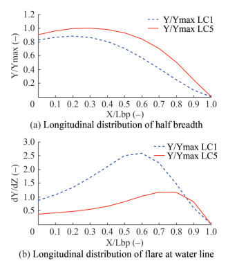
The study conducted by Paulling and Rosenberg (1959) investigated the stability of ships in calm water. Their work took into account the influence of non-linear second-order terms and coupling terms in the equation of motion. By solving the Mathieu Equation theoretically, they identified the existence of instability caused by non-linear coupling. The experimental tests, which coupled heave and roll motion, confirmed their findings. However, the researchers suggested that the coupling effect should incorporate more than two degrees of freedom. For several years, the parametric roll was considered only a theoretical concern until the APL China container ship experienced it in 1998. Following the accident, many scholars became intrigued by this phenomenon. Neves et al. (1999) conducted experimental and numerical investigations to examine the influence of different stern shapes on parametric rolls in fishing vessels. The study found that the transom stern resulted in a higher parametric roll amplitude compared to the round stern. This was attributed to a significant difference in the longitudinal flare distribution (dY/dZ) between the two stern shapes, which caused a different roll excitation. Francescutto (2001) conducted an experimental investigation to explore the possibility of parametric roll in a destroyer model when sailing into headseas. The study also calculated the roll damping through a roll decay test conducted in calm water with forward speed. However, the impact of waves on roll damping was not considered. Francescutto's findings demonstrated a potential risk for ships with relatively low roll periods at this heading (head waves). France et al. (2003) conducted a numerical study using FREDYN, a nonlinear, time domain ship motion simulation program developed by MARIN based on Hooft (1987), and LAMP (Large Amplitude Motion Program) based on Lin and Salvesen (1997) code to investigate the influence of stern and bow flare of Series 60 hull form on parametric roll amplitude. Results showed that ships with stern and bow flare have a higher parametric roll amplitude than those with bow flare of 0°, with the roll amplitude increasing as the bow flare increases.
Spanos and Papanikolaou (2006) investigated the occurrence of parametric roll in fishing vessels through time-domain numerical simulations in head waves. Their simulations utilised potential theory and considered non-linear terms in 6 degrees of freedom (6 DoF), with viscous effects incorporated through a semi-empirical linear or quadratic roll velocity model. The study demonstrated that the amplitude of the roll was influenced by the effect of wave amplitude on the parametric roll. Spanos and Papanikolaou (2007) studied the occurrence of parametric roll in two different types of ships, a fishing boat and a Ro-Ro vessel, in head waves using numerical simulations. The study results showed a difference in the occurrence of parametric roll between the two ships. The fishing vessel experienced a parametric roll at the lowest wave amplitude investigated in the study (0.6 m out of the highest amplitude, 1.4 m). In comparison, the Ro-Ro ship began experiencing parametric roll for wave heights from 4 m up to 6 m. Sadat-Hosseini et al. (2010) studied the ONR Tumblehome surface combatant to investigate the parametric roll phenomenon using a non-linear dynamics approach, EFD, and CFD, with and without bilge keel. The CFD method was used for the first time by Hosseini (2009) to predict parametric roll, as well as other modes of stability issues. The study revealed that the CFD results for the parametric roll were higher than the EFD results, although there was an agreement in trend between the two sets of results.
Riberio e Silva et al. (2010) presented a simple method to determine if a container ship is susceptible to parametric roll based on ABS guidelines. The study evaluated susceptibility criteria for two container ships. Miller's method (Miller, 1974) was used to calculate roll damping. Then, a numerical method was employed to simulate parametric roll cases in the time domain. Riberio e Silva et al. (2010) aimed to predict the amplitude of the roll motion. Based on this research, the ABS guidelines were found to be an adequate and efficient way to identify the occurrence of parametric roll.
Neves et al. (2011) investigated the influence of vessel speed and wave amplitude in regular head waves on roll response using two different stern shapes based on experimental and numerical methods. Fishing boats may experience different speeds to maintain their position in rough weather. The study concluded that vessel speed influenced the roll amplitude, with an asymmetrical pattern in the roll response. Park et al. (2013) conducted a sensitivity analysis of computational results of parametric roll in regular and irregular waves. Their research involved two container ships as case studies. The impulse-response-function (IRF) and 3D Rankine panel methods were used to simulate parametric roll in regular waves. The study showed a good agreement compared to Mathieu equation-based solutions. Galbraith and Boulougouris (2015) studied the parametric roll prediction of the Tumblehome model using the Star-CCM+ software. In their simulations, a different initial heel was applied, first, by setting an initial angular velocity of 0.1 rad/s and second, by shifting in the transverse centre of gravity by 0.001 48 m to starboard. Based on their findings, the second one accelerated the occurrence of the parametric roll by 20 s compared to the first, and the roll amplitude was slightly smaller.
Zhou et al. (2016) developed a hybrid method to predict the parametric roll of the C11 container ship. The method involved determining the damping coefficient from experimental data and a CFD method using free and forced roll decay, which was then used to predict the parametric roll based on potential theory. The results of the hybrid method were compared to the non-linear dynamics approach (used as a second check of Level 2 criteria by IMO) and CFD simulation and showed good agreement. Schumacher et al. (2016) conducted a study on the occurrence of parametric roll on a container ship, utilising both numerical and experimental approaches in regular and irregular wave conditions. Roll damping was evaluated through forced rolling tests, with both linear and nonlinear methods employed. The nonlinear time domain model was found to be in good agreement with the experimental test results. Lu et al. (2016) conducted a study on the relationship between parametric roll and added resistance. They expanded Mauro's theory (1963) for added resistance in head seas to examine the impact of parametric roll on added resistance using potential theory. The study included an experimental test to compare the numerical results, which showed agreement. The study found that the viscous roll damping affects the added resistance, and the effect becomes more significant as the parametric roll amplitude increases. Ma et al. (2018) studied the parametric roll phenomenon of a C11 container ship using experimental and numerical methods. The study also investigated the effects of draft, speed, and wave amplitude. The study showed that the parametric roll amplitude is not a linear function of wave steepness, with an initial increase followed by a gradual decrease. Additionally, the wave steepness that results in the maximum amplitude of parametric roll varies at each Froude number.
Zhou (2019) examined a hybrid approach to forecast the occurrence of parametric roll. The damping factor was determined through both CFD simulation and an experimental test. The results demonstrated that the direct CFD approach was more accurate than the hybrid method, as the fully non-linear viscous flow improved the hydrodynamic force prediction and critical wave steepness. Ghamari et al. (2020) conducted a study on the parametric roll of Norwegian fishing vessels in regular waves using numerical and experimental methods. The experimental tests were carried out with and without forward speed at different wave frequencies and steepness, and the roll damping was determined through roll decay tests. The numerical method involved using radiation and diffraction potentials at zero speed, followed by utilizing the results obtained by the strip theory based on Salvesen, Tuck and Faltinsen (STF) method. The study investigated a wide range of simulation conditions, with most cases showing consistent steady roll amplitude between experimental and numerical results. However, some discrepancies were observed in a few cases close to the instability border. Liu et al. (2021) utilised a CFD simulation to investigate the parametric roll of an ONR Tumblehome in both model and full scale. Their study revealed that the scale effect in parametric roll is negligible, as the difference is minimal. The presence of a bilge keel in the ship was found to be effective in reducing the amplitude of the parametric roll. In a subsequent study, Liu et al. (2022) examined the influence of liquid sloshing on the parametric roll of an ONR Tumblehome. Their research found that sloshing affects the natural roll frequency, decreasing the roll amplitude when the phase difference between the ship motion and sloshing is 180°. Zhou et al. (2022) investigated the vulnerability of the Offshore Research Vessel (ORV) to parametric roll caused by the extended low weather deck. They did not only examine the amplitude of the parametric roll but also the GZ curve, which they compared to experimental test results from previous studies. Additionally, the study investigated the non-linear water-on-deck phenomenon that occurs during parametric roll.
Sea area and season where and when the ship operates also influence the vulnerability to the parametric rolling of the ship. Hashimoto and Furusho (2022) investigated this issue in a C11-class container ship and a pure car and truck carrier. The results showed that Centre-North Pacific is the worst environmental condition for both ships. It also revealed that the winter season has a ten times higher failure index compared to summer. Another of interest in parametric roll study had been investigated by Maruyama et al. (2023). Their study investigates how to estimate roll acceleration with probability density function. Later, Liu et al. (2023) evaluated the second level of vulnerability criteria of parametric roll for C11 container ships with stochastic stability theory. Then, the results were compared with the stability criteria proposed by IMO. The proposed method gives more accurate results compared to IMO.
The majority of existing literature has verified a proposed numerical approach to predict parametric roll (PR) and helped to understand its behaviour. A discussion of various techniques has been presented. Several researchers have investigated the PR behaviour concerning wave steepness, wave amplitude, vessel speed, wave heading, and GM. However, there has been limited exploration of PR based on case studies of small fishing boats. To the best of our knowledge, no research has been conducted on the parametric roll of small fishing boats utilising fully non-linear unsteady RANS CFD simulations, particularly in different loading conditions that accurately represent fishing boat operations.
This study examines the impact of different loading conditions on a small fishing boat, which can alter the natural roll period, roll damping, and restoring moment values. The study investigates the influence of displacement and GM/KM ratio on GM Ratio and its effects on roll, pitch, and heave amplitude. The research also considers the effect of vessel shape and the distribution of longitudinal flare on the waterline. This phenomenon is unique to fishing boats since their loading condition changes continuously during operation. Furthermore, the natural roll frequency of small boats is low and may be close to the wave period, leading to the occurrence of parametric roll. The findings of this study are believed to provide valuable information to fishing vessel operators on optimal fish placement after catching them.
A CFD approach was chosen in this study as a method to predict the amplitude of parametric roll phenomenon on a small fishing boat because of its high accuracy. To enhance the efficiency of the time-domain simulation, the wave steepness and vessel speed that trigger the PR in each load case were identified early on, using ABS recommendations (American Bureau of Shipping (ABS), 2019). This study also investigated the impact of viscosity by comparing various y+ strategies. The diffusion term in the URANS method encompasses viscous effects, resolved using the turbulence model in the boundary layer region. As subsequently demonstrated, accounting for viscous effects is crucial to predict the roll motion accurately.
3 Ship geometry and loading conditions
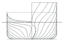
In this paper, a five-metre-long traditional fishing boat from Indonesia was used. This fishing boat underwent geometric optimisation by Tezdogan et al. (2018). Later, Liu et al. (2019) designed a bilge keel for this boat. A body plan of the fishing boat is shown in Figure 1, and the main dimensions are given in Table 1. The latest investigation into this fishing boat was carried out by (Iqbal et al., 2023), who investigated the operability analysis under different loading conditions.
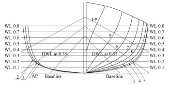 Figure 1 Body plan of the research object (Liu et al., 2019)Table 1 Main dimensions of the fishing boat (Tezdogan et al., 2018)
Parameter Value Length between perpendicular, LBP (m) 5.000 Breadth at the water line, B (m) 1.934 Depth to 1st deck, D (m) 1.196 Loaded draft, T (m) 0.350 Displacement, Δ(t) 1.858 Block coefficient, Cb 0.537 Mid-boat section coefficient, Cm 0.764 Wetted surface area, Aw (m2) 10.201 Maximum Froude number, Fr 0.590 Iqbal et al.'s (2023) research examined five distinct loading conditions, representing a fishing vessel's operational conditions. These conditions ranged from the boat being empty at the port to gradually filling the fish tank to 50% and 100% capacity. Furthermore, in each half and full-loading condition, the fish were placed on both the deck and below the deck. This approach was taken because fishermen often put their catch on the deck before depositing them inside the tank. This paper, however, uses a different loading condition from Iqbal et al.'s (2023) study, as presented in Table 2, to investigate the parametric roll phenomenon. The LCG is measured from AP, while KG is measured from baseline.
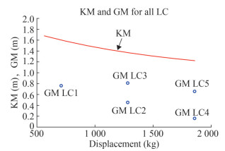
Table 2 Loading condition of the fishing vessel operation (Iqbal et al., 2023)Load case Description Ship weight (kg) LCG (m) KG (m) GM (m) 1 Empty load of fish 712.00 1.550 0.844 0.763 2 Half load of fish, upper deck 1 285.00 1.751 0.914 0.456 3 Half load of fish, below deck 1 285.00 1.751 0.557 0.813 4 Full load of fish, upper deck 1 858.00 1.828 1.064 0.163 5 Full load of fish, below deck 1 858.00 1.828 0.57 0.657 4 Methodology
4.1 Flowchart
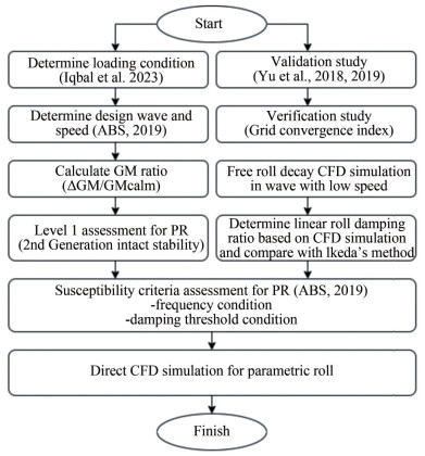
The simulation flowchart is presented in Figure 2, where the steps involved in conducting a CFD simulation for the KCS model are shown on the right-hand side. First, a fine mesh configuration was simulated using two different y+ strategies. Then, steady roll amplitudes obtained using low and high y+ meshing strategy were compared to the experimental result obtained from the parametric roll test of the KCS model studied by Yu et al. (2018; 2019). This uses an estimate of the discretisation uncertainty obtained through the Grid Convergence Index (GCI) method, which forms the verification study. Following this, the set-up of CFD simulation of the KCS model was done for both free roll decay simulation and direct CFD simulation on parametric roll. The free roll decay results, the linear roll damping ratio, were used as an input in susceptibility criteria assessment. The linear roll damping obtained from CFD calculations was also compared to Ikeda's method, which was calculated in the ShipX software with the same conditions as CFD. The viscous roll damping in ShipX software is determined from an empirical formula for roll motions. The components of this formula are frictional shear stress on the hull surface (Kato, 1957), eddy damping (Ikeda et al., 1977), lift damping (Himeno, 1981) and the bilge keel damping (Ikeda, 1979). The latter component is not included because in this study the boat has no bilge keel.
The left-hand side of the flowchart starts by determining the loading conditions, as shown in Table 2. The ABS (2019) recommendation is used to determine the design wave and vessel speed for a given loading condition. This design wave is then used to calculate the GM variation as the wave crest moves from the bow to the stern. The resulting GM Ratio is then used to perform the Lv1 Parametric Roll Assessment of Second Generation of Intact Stability (SGIS) and to assess the susceptibility criteria, following the ABS' (2019) method. Finally, after determining the design wave and boat speed in each load case and having done the CFD setup, the direct CFD simulations of the fishing boat to investigate a parametric roll can be carried out.
4.2 Determination of the design wave and vessel speed
The ABS (2019) guidelines recommend using a wavelength equal to the ship length and Table 3 to determine the wave height based on the relationship with its length. The table shows that the wave steepness ratio, Hw/λ (where Hw is the wave height and λ is the wavelength), increases when the wavelength decreases. In this particular study, the fishing boat's length is 5 m, so the wavelength λ is also 5 m. According to the table, the Hw/λ ratio used was supposed to be 0.12 (for the lowest wavelength), resulting in a wave height of 0.6 m. However, this ratio is too high for a 5-metre fishing boat, and it would cause wave breaking. Therefore, a lower Hw/λ ratio of 0.06 was used, resulting in a wave height of 0.3 metres.
Table 3 Wave height information according to the Wave Scatter Data from IACS RecommendationWavelength, λ (m) Wave height, Hw (m) Hw/λ 50 5.9 0.12 100 11.6 0.12 150 14.2 0.09 200 15.1 0.08 250 15.2 0.06 300 14.6 0.05 350 13.6 0.04 400 12.0 0.03 450 9.9 0.02 Equation (1) from ABS (2019) was employed to determine the velocity of the boat (VPR, in knots) that leads to a parametric roll. In Equation (1), If 2ωm > ωw (where ωw is the wave frequency and ωm is the mean frequency) the parametric roll phenomenon will be expected in head waves. Conversely, if 2ωm < ωw the parametric roll will be expected in stern waves, which can be determined based on the wavelength. ωm is the mean frequency that obtained from GMm by calculating the stability in longitudinal wave, explained in the following subsection.
$$ V_{\mathrm{PR}}=\frac{19.06 \times\left|2 \omega_m-\omega_w\right|}{\omega_w{ }^2} $$ (1) 4.3 Calculation of the GM ratio (level 1 assessment of PR)
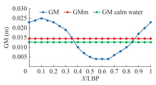
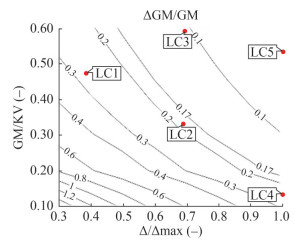
Using the design wave determination procedure described earlier, the wave crest (X) location was shifted along the ship length (LBP) to calculate the GM. Maxsurf Stability software was employed to calculate this step, resulting in GMmax, GMmin, GMm, and GMa, as shown in Figure 3. Here, GMmax and GMmin are the maximum and minimum GM values, while GMm is mean of GM, where GMm = 0.5(GMmax + GMmin), and GMa is the amplitude of GM calculated as 0.5(GMmax − GMmin). GMa is also referred to as ΔGM and is used to calculate Level 1 vulnerability criteria of Parametric Roll in the Second Generation of Intact Stability (SGIS), as shown in Equation (2).
A ship is predicted to experience parametric roll if ΔGM/GMcalm > RPR, where RPR is a semi-empirical factor based on the basic geometrical characteristics of a vessel, such as L, B, and midship coefficient (Cm). The equation is stated in IMO (2008), which is highly sensitive to bilge keel area, Ak. When there is no bilge keel installed on the vessel, RPR is set as 0.17. In the present investigation, the computation proceeds to the Direct Stability Assessment (DSA) stage instead of Level 2, in the event of a failure in Level 1 assessment, when ΔGM/GMcalm > RPR. This decision is taken considering the utilisation of the computational fluid dynamics (CFD) technique to simulate the amplitude of parametric roll.
$$ \frac{\Delta \mathrm{GM}}{\mathrm{GM}_{\text {calm }}} \leqslant R_{\mathrm{PR}} $$ (2) The result of Equation (1) (vessel speed) and Equation (2) (Lv 1 assessment of PR) are shown in Tables 4 and 5, respectively. As Table 4 indicates, the speeds at which PR is triggered vary for each load case. The wave direction for all load cases is head waves, except for load case 4, which involves following waves. In Table 5, all load cases except LC3 and LC5 failed to satisfy the Level 1 assessment for PR, thereby necessitating progression to Level 2 assessment. Nonetheless, this study undertakes a DSA, which leverages Computational Fluid Dynamics (CFD) simulation to estimate the amplitude of PR, instead of Level 2 assessment.
Table 4 Result of vessel speed and wave direction for λ = 5.0 m and Hw = 0.3 m based on Eq. 1Load case Tn(s) Boat speed, VPR (m/s) Wave direction Te (s) Te/Tn 1 2.00 2.37 Head waves (2ωm > ωw) 0.968 0.48 2 2.00 1.33 Head waves (2ωm > ωw) 1.212 0.61 3 1.60 2.85 Head waves (2ωm > ωw) 0.886 0.55 4 4.38 0.35 Following waves (2ωm < ωw) 2.046 0.47 5 1.57 2.36 Head waves (2ωm > ωw) 0.970 0.62 Table 5 The results of Level 1 SGIS (Eq. 2)Load case ΔGM GMcalm ΔGM/GMcalm RPR Status 1 0.419 0.763 0.261 0.17 Failed 2 0.252 0.456 0.184 0.17 Failed 3 0.145 0.813 0.106 0.17 Pass 4 0.271 0.163 0.221 0.17 Failed 5 0.071 0.657 0.058 0.17 Pass 4.4 The susceptibility criteria of parametric roll
Prediction of parametric roll in regular waves can be accomplished using the Mathieu equation. This equation can be deconstructed by considering a ship moving in waves with forward speed. As the ship moves through the waves, the GM of the ship changes in response to the location of the wave crest and trough.
The change of GM can be simplified with the sinusoidal waves as shown in Equation (3). By substituting Equation (3) to the equation of 1 DOF of damped free roll motion, one arrives at Equation (4), where ωm2 = Δ.GMm/(Ixx + IA.xx) and ωa2 = Δ.GMa/(Ixx + IA.xx). Then, the parameter ωet can be replaced with τ, a notation to normalise Equation (4) by dividing it by ωe2 resulting in Equation (5). The ζ symbol in Equation (4) is the defined as a damping ratio, the ratio between the linear damping coefficient of the roll (B) to its critical damping (Bc).
The present paper determines the linear roll damping for every load case from free roll decay simulation. A speed of 0.2 m/s was selected in the simulation to produce τ or ωet. High speeds were avoided as they may increase the roll damping coefficient (B) and reduce the roll motion.
The condition of fishing vessels when determining the roll damping using CFD simulation is that the vessel is non-stationary and in waves. The first reason for this is to obtain the roll damping as realistic as possible. When the fishing boat experiences the parametric roll, it occurs in waves (not in calm water) and at non-zero speed condition. The second reason is the roll damping obtained from waves is mostly higher than in calm water, as reported by Rodríguez et al. (2020). Therefore, it would be overestimated if we use the roll damping based on calm water values.
The result of linear roll damping was subsequently compared to that obtained from Ikeda's method, which was computed using ShipX software under the same conditions as the CFD simulation.
To eliminate the second term (linear damping) in Equation (5), the solution of 1 DOF of damped free roll motion (Equation (6)) is used and results in Equation (7). This equation is referred to as the Mathieu equation. The common form of the Mathieu equation is shown in Equation (8).
$$ \mathrm{GM}=\mathrm{GM}_m+\mathrm{GM}_a \cos \left(\omega_e t\right) $$ (3) $$ \frac{\mathrm{d}^2 \phi}{\mathrm{d} t^2}+\left(2 \zeta \omega_n\right) \frac{\mathrm{d} \phi}{\mathrm{d} t}+\left(\omega_m{ }^2+\omega_a{ }^2 \cos \left(\omega_e t\right)\right) \phi=0 $$ (4) $$ \frac{\mathrm{d}^2 \phi}{\mathrm{d} \tau^2}+\left(2 \frac{\zeta \omega_n}{\omega_e}\right) \frac{\mathrm{d} \phi}{\mathrm{d} \tau}+\left(\frac{\omega_m^2}{\omega_e^2}+\frac{\omega_a^2}{\omega_e^2} \cos (\tau)\right) \phi=0 $$ (5) $$ \phi(\tau)=x(\tau) \cdot e^{-\mu \tau} $$ (6) where μ = ζωn/ωe
$$ \frac{\mathrm{d}^2 \phi}{\mathrm{d} \tau^2}+\left(\frac{\omega_m{ }^2}{\omega_e{ }^2}-\frac{\left(\zeta \omega_n\right)^2}{\omega_e{ }^2}+\frac{\omega_a{ }^2}{\omega_e{ }^2} \cos (\tau)\right) \phi=0 $$ (7) $$ \frac{\mathrm{d}^2 x}{\mathrm{~d} \tau^2}+(p+q \cos (\tau)) x=0 $$ (8) where $ p=\frac{\omega_m{ }^2}{\omega_e{ }^2}-\frac{\left(\zeta \omega_n\right)^2}{\omega_e{ }^2}=\frac{\omega_m{ }^2}{\omega_e{ }^2}-\mu^2, q=\frac{\omega_a{ }^2}{\omega_e{ }^2}$
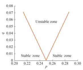
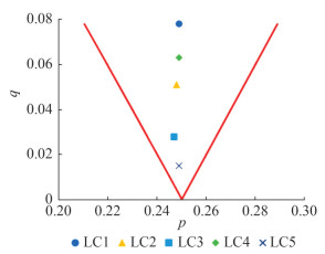
There are two susceptibility criteria based on ABS after p and q are determined. First, the frequency of parametric excitation (encounter wave frequency) should be about double of natural roll frequency (ωe ≈ 2ωn) or the encounter wave period should be about a half of natural roll period (Te ≈ 0.5Tn). The frequency condition of susceptibility criterion is shown in Figure 4 and Equation (9). The boundary line in Figure 4 is determined from Equation (9) and is sourced from ABS (2019). Based on these, the ship is considered susceptible to parametric roll if the point obtained from the combination of p and q lies inside the unstable zone.
$$ \frac{1}{4}-\frac{1}{2} q-\frac{1}{8} q^2+\frac{1}{32} q^3-\frac{1}{384} q^4 \leqslant p \leqslant \frac{1}{4}+\frac{1}{2} q $$ (9) $$ \frac{\zeta \omega_n}{\omega_e}<q \cdot k_1 \cdot k_2 \sqrt{1-k_3{ }^2} $$ (10) where k1 = 1 − 0.187 5q2, k2 = 1 002p + 0.16q + 0.759, k3 =$ \frac{q^2-16+\sqrt{q^4+352 q^2+1024 p}}{16 q}$
Even though the first criterion is satisfied, the parametric roll can appear because roll damping plays an important role. If the roll damping is sufficiently high, the parametric roll caused by changing stability in waves will not develop. However, if the roll damping is insufficient to reduce the roll amplitude significantly, then parametric roll will develop. Therefore, the second susceptibility criterion from ABS is about the roll damping threshold. The ship is susceptible to parametric roll if the effective damping (ζωn/ωe) of the ship is smaller than the damping threshold $\left(q \cdot k_1 \cdot k_2 \sqrt{1-k_3^2}\right) $, as shown in Equation (10).
4.5 Numerical set-up
This section describes the numerical set-up used in this study. The commercial CFD software, Siemens Star-CCM+ version 16.04, was used to carry out all simulations. In integral form, the averaged continuity and momentum equation were solved by discretising them using the Finite Volume Method (FVM) sequentially by using the Segregated Flow Solver. This solver utilises a pressure-velocity coupling algorithm. This study used the Semi-Implicit Method for Pressure Linked Equations (SIMPLE) algorithm. The convective term was solved based on the second-order convection scheme, while first-order temporal discretisation was used to solve time discretisation.
4.5.1 Governing equation
Reynold Averaged Navier Stokes (RANS) equation models the fluctuating velocity field in an averaged manner. The averaged continuity and momentum equation for incompressible flow with surface forces without body force are shown in Equation (11) and (12), respectively.
$$ \frac{\partial\left(\rho \bar{u}_i\right)}{\partial x_i}=0 $$ (11) $$ \frac{\partial\left(\rho \bar{u}_i\right)}{\partial t}+\frac{\partial}{\partial x_j}\left(\rho \bar{u}_i \bar{u}_j+\rho \overline{u_i^{\prime} u_j^{\prime}}\right)=-\frac{\partial \bar{p}}{\partial x_j}+\frac{\partial \bar{\tau}_{i j}}{\partial x_j} $$ (12) where ρ is fluid density, uiuj and p are mean velocity vector and mean pressure in Cartesian xi. $\overline{u_i^{\prime} u_j^{\prime}} $ is the Reynolds stresses. For the eddy-viscosity model is shown in Equation (13). τij is mean viscous stress tensor, as shown in Equation (14).
$$ -\rho \overline{u_i^{\prime} u_j^{\prime}}=2 \mu_t S_{i j}-\frac{2}{3} \rho \delta_{i j} k $$ (13) $$ \bar{\tau}_{i j}=\mu\left(\frac{\partial \bar{u}_i}{\partial x_j}+\frac{\partial \bar{u}_j}{\partial x_i}\right) $$ (14) μt is the turbulent (or eddy) viscosity, Sij is the mean strainrate tensor in which $ S_{i j}=\frac{1}{2}\left(\frac{\partial \bar{u}_i}{\partial x_j}+\frac{\partial \bar{u}_j}{\partial x_i}\right)$, μ is the dynamic viscosity, δij is Kronecker delta, where δij = 1 if i = j otherwise δij = 0. Finally, k is the turbulent kinetic energy, as shown in Equation (15).
$$ k=\frac{1}{2} \overline{u_i^{\prime} u_i^{\prime}}=\frac{1}{2}\left(\overline{u_x^{\prime} u_x^{\prime}}+\overline{u_y^{\prime} u_y^{\prime}}+\overline{u_z^{\prime} u_z^{\prime}}\right) $$ (15) 4.5.2 Turbulence model and near-wall modelling
The fluid flow around the full-scale hull is turbulent. We can identify this based on the Reynolds number. In this study, the small turbulent fluctuations are averaged or filtered, opting for the Reynolds-Averaged Navier-Stokes (RANS) approach instead. The Shear-Stress Transport (SST) (Menter, 1994) model was used, which combines a k − ɛ model in the far field with a k − ω model near the wall.
The no-slip wall is a boundary condition that is a source of vorticity in most flow problems (Siemens, 2022). The ship hull is defined as the wall for all CFD simulations in the naval architecture field. There is a region near the wall called the boundary layer. It is important to predict the fluid flow and turbulence in this region as accurately as possible.
Based on the non-dimensional wall distances (y+), the boundary layer is divided into three regions, namely, the viscous sublayer (y+ < 5), the buffer layer, (5 < y+ < 30), and the log layer (y+ > 30). The buffer layer, which is typically avoided, is transitional between the viscous sublayer and the log layer. Neither the wall function nor the near-wall treatment can be used in this region. The all y+ treatment scheme in Star CCM+ package was used in this simulation to treat the boundary layer region either in low y+grids (when y+ < 5) or in high y+ grids (when y+ > 30).
Determining the number of near-wall layers is essential to obtain the desired y+ effectively. The procedure to determine the number of these layers in this study was based on Terziev et al. (2022). By initially computing the friction coefficient, Cf, using ITTC correlation line (Equation (16)), the shear wall stress, τw can subsequently be ascertained (Equation (17)). Here Re denotes the Reynolds number and V denotes the vessel's forward speed. Afterwards, the first layer thickness (2Δy) can be calculated using Equation (18), where v is the kinematic viscosity and $ u_t=\sqrt{\tau_w / \rho}$ is friction velocity. It should be noted that Δy is the distance between the wall to the first cell centre. Thus, the first layer thickness is equal to 2Δy.
Finally, the number of prism layers, n, can be calculated using Equation (19), where S is the stretch factor, expressing the ratio of the thickness of any two adjacent cell layers, and δ is the distance over which near-wall layers are distributed. The current research reported in this paper used the stretch factor of 1.2. The specific distance, δ, was determined by modelling a fraction of the flat plate equivalent turbulent boundary thickness δ = 0.382 L/Re1/5.
$$ C_f=0.075 /\left(\log _{10} R e-2\right)^2 $$ (16) $$ \tau_w=0.5 \rho V^2 C_f $$ (17) $$ \varDelta_y=y^{+} v / u_t $$ (18) $$ n-\log _{10}\left(1-\frac{\delta(1-S)}{2 \varDelta_y}\right) / \log _{10}(S) $$ (19) 4.5.3 Capturing free surface
For multiphase simulations, the interface between two phases can be captured using different techniques. There are three methods that is available in most of CFD code nowadays, which are: 1) surface fitting/mesh deformation, 2) surface capturing, and 3) level set (Wackers et al., 2011).
The present study employs the Volume of Fluid (VoF) method. This technique included as the family of surface capturing method, as stated in Siemens (2022). The VoF approach, first introduced by Hirt and Nichols (1981), differentiates between the two fluid phases (water and air) by assigning a scalar value between 0 and 1 to each cell, representing the volume fraction (αi) of a particular fluid in that cell. The volume fraction αi is defined as Voli/Vol, where Voli is volume of phase i and Vol is the volume of the cell.
For example, a cell that contains only water, αi is be assigned as 1. Likewise, a cell that contains only air, αi is be assigned as 0. Based on this scalar value, the interface between two fluid phases (the cells contain water and air) can easily be defined as the collection of cells with a volume fraction αi of 0.5.
The algorithm of the surface capturing method (VoF) is generally described in Wackers et al. (2011):
1) Set the initial flow field quantities (Q0) at t = t0.
2) Set the new time step, where t = t + Δt.
3) Start the iteration with Q = Q0.
4) Calculate the volume fraction for each fluid phase and update the fluid properties ρ and μ.
5) Compute the turbulence quantities from Q in step 3.
6) Solve the momentum equation to determine the new velocities.
7) Solve the pressure equation to determine the new pressure field.
8) Update and correct the new velocity based on the new pressure filed.
9) If the residual is still high, go to step 3 and update the iteration in the same time step.
10) Go to step 2 and update the time t.
In step 4 (calculating the volume fraction in transport equation), the density of the fluid in each cell is defined as $\rho=\sum_i \rho_i \alpha_i $, and the viscosity is defined as $ \mu=\sum_i \mu_i \alpha_i$, where ρi and μi are the density and viscosity of phase i. The total volume fraction for all phases in one cell must be one. $\sum\limits_{i=1}^N \alpha_i=1 $, where N is the total number of phases.
The high-resolution interface capturing (HRIC) scheme in the software package proposed by Muzaferija (1998), was employed to maintain a sharp interface between the fluid phases. This scheme is suitable for tracking sharp interfaces such as those formed between water and air.
Zhang et al. (2023) developed a new theory that can accurately predict the dynamics of a bubble, such as bubble oscillation, migration, and collapse due to pressure pulse. In the future, the theory can be more explored for the multiphase flow-related problem, such as the free surface that is related to ship hydrodynamics.
4.5.4 Simulation of ship motions
The employed solver, Star CCM+, uses the Dynamic Fluid Body Interaction (DFBI) module to simulate the motion of a rigid body. This module allows a body to respond to forces and moments applied by the physics continuum or any additional user-defined force or moment (Siemens, 2022). The restoring arm variation is not only influenced by the waves themselves, but also by the coupling between heave, pitch, and roll (Neves and Rodríguez, 2006). Thus, the DFBI module was utilised in this study to capture three degrees of freedom of the boat when moving on the wave, which is pitch, roll and heave. The DFBI module also computes exciting forces, moments, and the gravitational force acting on the hull and solves the governing equation of motion to determine the new position of the rigid body at each time step. In this paper, a selected DFBI module option was multi-body motion. It allows the boat to move in 3-DoF, as mentioned above.
4.5.5 Computational domain and coordinate system
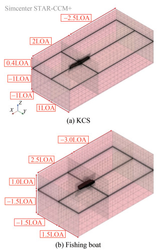
The computational domain size for KCS model covers from − 2.5LOA < x < 2LOA in length and − 1LOA < z < 0.4LOA for height, and − 1LOA < y < 1LOA in width. There is a difference in hull shape between the KCS and the fishing boat, where the KCS is more slender than the fishing boat. Specifically, the L/B ratio of the KCS is 7.14, whereas that of the fishing boat is 2.59. As the ratio of the fishing boat is lower, a larger computational domain is required than for the KCS, specifically − 3.0LOA < x < 2.5LOA in length and − 1.5LOA < z < 1.0LOA for height, and − 1.5LOA < y < 1.5LOA in breadth.
Figure 5 displays the computational domains for the KCS model and the fishing boat. The size of computational domains for other similar CFD studies in the literature is shown in Table 6. It should be noted that the domain size was reversed for LC4. In this case, the downstream was positioned behind the boat, while the upstream was situated in front of the boat.
Table 6 Computational domain size of similar previous studiesReference Upstream Downstream Top Bottom Transverse (Sadat-Hosseini et al., 2010) 0.5L 2.0L 0.25L 1.0L 1.0L (Ma et al., 2018) 2.0λ 4.5λ 1.5λ 2.5λ 2.5λ (Liu et al., 2021) 1.0L 3.0L 0.4L 1.0L 1.0L In this simulation, the coordinate system is defined such that the X direction aligns with the longitudinal axis, parallel to the ship length, with the zero-point coinciding with the AP and the positive direction oriented towards the FP. The Y axis aligns with the transversal direction, with the zero-point at the ship's centre line and the positive direction toward the port side. The vertical direction corresponds to the Z axis, with the zero-point located at the calm water free surface. The positive direction is upward, and the negative direction is downward.
4.5.6 Boundary condition
For boundary condition set-up, the hull surface is set as a no-slip wall, which means the fluid velocity in the hull surface is zero. All boundary conditions on the rectangular domain sides are set as velocity inlet, except for the downstream side, which is the pressure outlet. This boundary type was the same as in Galbraith and Boulougouris (2015), Ma et al. (2018) and Liu et al. (2021), where the downstream boundary was set as a pressure outlet, and remains boundary as a velocity inlet. These boundary conditions are reversed for LC4.
For the inlet boundary, the fifth-order VOF Wave modules were used to represent fluid in the computational domain with the wave. The forcing method was applied on the Inlet, outlet, and right and left side boundaries. This method forces the fluid properties and the volume fraction of water in the forcing zone to be what the user inputs in the boundary condition. In this case, the forcing zone is forced to produce the fifth-order wave defined in the inlet boundary condition. Technically, the free surface contour in the forcing zone is unaffected by the ship's speed and motion. This means that the wave reflection from the boundaries can be avoided. The forcing length was set as 1 LOA (2.415 m) from inlet and outlet boundaries and 1.0 m from the left and right-side boundaries.
4.5.7 Mesh generation
The automatic meshing facility in Star CCM+ was used to generate mesh based on the cartesian cut-cell method. Trimmed cell mesher and surface remesher are applied to generate a volume grid consisting of hexahedral cells and refine it to be a high resolution of rectangular mesh on a surface. For the verification study, the influence of two different y+ values on the amplitude of parametric roll were compared, namely y+ < 1 and 30 < y+ < 100. Using the method described in Section 4.5.1, twelve layers of prismatic cells were used with the first grid distance of 4.579 × 10⁻⁵ m for a 2.3 m KCS model to ensure the averaged y+ < 1 over wetted surface area (WSA).
On the other hand, to set a targeted y+=30‒100, one layer of the prismatic cell was used with the first grid distance of 3.625×10⁻³ m. The hull boundary layer for the fishing boat simulations was set to 17 layers for the highest Reynolds number (LC 3) to ensure y+ < 1. This same number of layers was used for all load cases except for LC 4, which used 15 layers since its Reynolds number was the lowest among all load cases.
The Star CCM+ software offers three mesh configurations to simulate rigid body motion: moving mesh, morphing, and overset mesh. Moving mesh involves moving all the mesh in the domain based on the body's movement, while morphing deforms the mesh around a moving body without moving the domain. On the other hand, overset mesh consists of two regions, the background and overset, where the overset mesh moves while the background remains static.
A comparison of these three methods on the resistance of planning hull was described by Yulianti et al. (2022). It is stated that computational time needed in the overset mesh is lower than moving mesh but higher from morphing mesh. However, for high amplitude roll, such as in this paper, the morphing mesh is not able to cover. Then, the best option to be used is overset mesh.
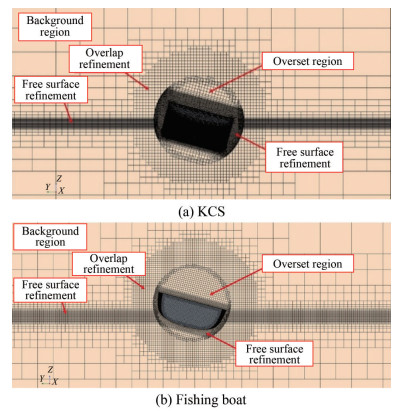
In this study, the overset mesh module was used. Mesh refinements were set in the free surface region. All simulation settings used in this study followed the ITTC (2011) recommendation, where longitudinal and transversal refinement at the free surface region are λ/80 and Hw/20 for the horizontal and vertical directions, respectively. The same mesh refinements were also applied to fishing boat simulations. Figure 6 shows the visualisation of two regions and mesh refinement of for both the KCS model and the fishing boat.
4.5.8 Determination of the time step
ITTC recommends a minimum of 100 time-steps per period for periodic phenomena, such as roll decay. In this study, the encounter period (Te) was used, which was approximately 1.002 s. According to ITTC's recommendation, the minimum time step should be 0.01. However, and a time step of 0.005 s was used for this CFD simulation, which is lower than ITTC's recommendation.
Meanwhile, according to Table 4, the minimum Te for fishing boat simulation is for LC3, which is 0.886 s. Therefore, the minimum time step recommended by ITTC is 0.008 8 s. However, for all load cases used in this simulation, the time step was set to 0.001 s, except for LC4, which used a time step of 0.007 s. The encounter frequency of LC4 was higher, 2.046 s, resulting in a minimum time step of 0.02 s, based on ITTC recommendations.
4.5.9 Total of computational time
All the simulation in this study was carried out using High Performance Computer (HPC), provided by Archie-West, by using 25 cores (CPUs). For four KCS simulations, the average computational time is 77 hours. This means that the total core hours for each simulation is 77 × 25, which is 1925 core hours for approximately 20 s of physical time.
For five simulations in determining roll damping of fishing vessels, the average of total computational time is 13 hours. Then, the total of each computational time is 13 × 25, which is 325 core hours for 8 s in physical times, except for Load Case 4 (20 s).
The average of computational time for parametric rolling simulation for small fishing vessels is higher. The average is 164 hours for each simulation to reach 20 s in physical time, except load case 4 (72 s). The total core hours then, 164 × 25, which is 4 100 core hours for each simulation.
4.6 Fast Fourier transform analysis
As the simulation is unsteady, its results are time-dependent and presented in the time domain. These results can be transformed into the frequency domain using Fast Fourier Transform (FFT) analysis to obtain quantitative insights.
$$ \varphi(t)=\varphi_0+\sum\nolimits_{n=1}^N \varphi_n \cdot \cos \left(\omega_n t+\gamma_n\right), n=1, 2, 3, \cdots $$ (20) where φn is nth harmonic amplitude and γn is the corresponding phase which can be determined by using Equation (21) and (22). The n value indicates the total cycles that used in FFT analysis. For example, in this study we used the last three cycles of the results of roll motion. Thus, the n value that used in Equation (20) is equal to 3.
$$ \varphi_n=\sqrt{a_n^2+b_n^2} $$ (21) $$ \gamma_n=\arctan \left(\frac{b_n}{a_n}\right) $$ (22) where
$$ a_n=\frac{2}{T} \int_0^T \varphi(t) \cdot \cos \left(\omega_n t\right) \mathrm{d} t $$ (23) $$ b_n=-\frac{2}{T} \int_0^T \varphi(t) \cdot \sin \left(\omega_n t\right) \mathrm{d} t $$ (24) $$ \varphi_0=\frac{1}{T} \int_0^T \varphi(t) \mathrm{d} t $$ (25) The 0th harmonic amplitude φ0 is the average value of the time history of φ(t).
5 Results and discussion
5.1 Verification
5.1.1 Reference data and condition
A verification study was carried out to measure the uncertainty obtained from the numerical results. This study covers a systematic verification for the KCS model scale with Lbp = 2.3 m under parametric roll condition (v= 0.4 m/s, λ/Lbp = 1.0, and H/λ = 0.02). The case is made the same as Yu et al. (2018, 2019), since they have the experimental data that can be used to compare numerical and experimental results. The body plan of KCS is shown in Figure 7. The main dimension of KCS model and simulation condition are shown in Table 7.
7(a) Main dimensions of the KCS model (1:100)Parameters Value Length between perpendicular, Lbp (m) 2.3 Breadth at water line, B (m) 0.322 Depth, D (m) 0.19 Loaded draft, T (m) 0.108 Displacement (kg) 52.31 Longitudinal centre of buoyancy, LCB from AP (m) 1.116 Height of centre of gravity, KG (m) 0.136 6 Metacentric height, GM (m) 0.012 7 0.324 2, Kxx/B, Kyy/Lbp, Kzz/Lbp 0.249 5, 0.246 5 Roll natural period, Tn (s) 2.16 7(b) Simulation conditionsParameters Value V (m/s) 0.40 Wavelength, λ/Lbp 1.00 Wave height/wavelength, Hw/λ 0.02 Te/Tn 0.464 The Grid Convergence Index (GCI) method was used to conduct the verification study. This approach is based on the Richardson extrapolation (1911) as described by Celik et al (2008). At least three solutions should be evaluated in terms of convergence behaviour. In this paper, both grid and time uncertainty were conducted in the same simulation with different refinement, namely coarse, medium, and fine configurations. This approach aligns with recommendations made by Burmester et al. (2020) and ensures that the achieved Courant number remains consistent across the solution triplet. In addition, the number of prism layers remains constant across the solution triplet while the distance over which near-wall layers are distributed is magnified accordingly to retain identical cell aspect ratios. The fine configuration was coarsened in terms of both for grid and time step simultaneously through the refinement ratio of r21 = 1.23 and the medium configuration was coarsened again into the coarse configuration by multiplying by the refinement ratio r32 = 1.24, following to Ravenna et al. (2022). It should be noted that the remaining simulations in this paper used the fine configuration.
Once three solutions are obtained, the difference between medium-fine and coarse-medium can be obtained using Equation (26) and Equation (27), where S1, S2, and S3 are the solution for fine, medium, and coarse configurations, respectively. Then, the convergence ratio, R, can be calculated using Equation (28). The value of convergence ratio categorizes the behaviour of the simulation with refinement into three types, monotonic convergence (0 < R < 1), oscillatory convergence (− 1 < R < 0), and divergence (|R| > 1). The order of accuracy, p, then can be calculated using Equation (29) iteratively, where r21 and r32 represent the medium-fine and coarse-medium refinement ratios, respectively. Finally, the GCI can be estimated based on Celik et al. (2008) by using Equation (30).
$$ \varepsilon_{21}=S_2-S_1 $$ (26) $$ \varepsilon_{32}=S_3-S_2 $$ (27) $$ R=\frac{\varepsilon_{21}}{\varepsilon_{32}} $$ (28) $$ p=\frac{1}{\ln r_{21}}|\ln | \frac{\varepsilon_{32}}{\varepsilon_{21}}|+q(p)| $$ where
$$ q(p)=\ln \left(\left(r_{21}^p-s\right) /\left(r_{32}^p-s\right)\right) \text {, and } s=\operatorname{sgn}\left(\varepsilon_{32} / \varepsilon_{21}\right) $$ (29) $$ \mathrm{GCI}=1.25\left|\frac{S_1-S_2}{S_1}\right| /\left(r_{21}^p-1\right) $$ (30) 5.1.2 Error comparison
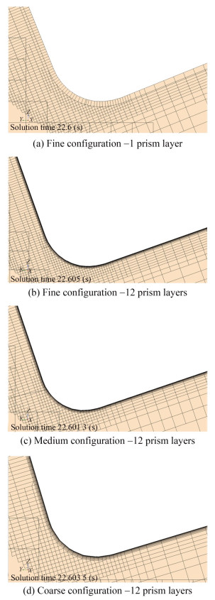
A study was carried out by comparing the CFD results of fine configuration with the experimental results. The results of CFD simulation on the parametric roll of 2.3 m KCS model were compared with the experimental results from Yu et al. (2018; 2019). A different wall treatment was used to investigate the viscous effect's influence on the amplitude of roll during parametric roll motions. Two y+ values were used, y+ = 30‒100 and y+ < 1. A varying number of prism layers, including both single layer and 12 prism layers, were implemented around the hull to obtain the different y+ values. The fine mesh configurations for two different total number of layers are shown in Figure 8.
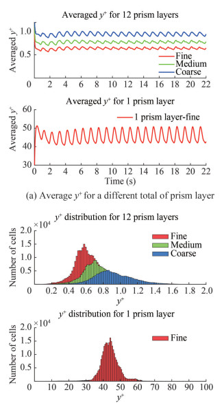
The obtained values of averaged y+ for the wetted surface area of the hull are presented in Figure 9. The single layer configuration resulted in a range of y+ values between 40‒55, while the 12-layer configuration produced values of y+ less than 1. To make it clearer, the distribution of y+ in every cell on the wetted surface cell is also presented. As previously stated, selecting different y+ values can affect the wall function implemented for turbulence resolution. Specifically, when y+ was between 30‒100, the logarithmic law region was employed to solve the boundary layer around the hull. In contrast, a viscous sublayer region was used when y+ was less than 1.
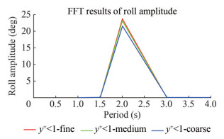
Fast Fourier Transform (FFT), as described in Equation (20), was used to transform the time series of roll amplitude into the frequency domain. This method was also used to quantify the amplitude of the roll. The time series results of the roll amplitude obtained from the CFD simulation are shown in Figure 10. Different y+ configurations were also compared to the experimental data from (Yu et al., 2018; Yu, 2019). The comparison with the experimental data is only based on the roll amplitude, as no time series data is available for other modes of motion for this test simulation. Then, the last three cycles from the present CFD results were used to transform the time domain results into the frequency domain using FFT because the amplitude was steady.
The FFT results of different y+ configurations are shown in Figure 11 and were compared with experimental results. The comparison results are shown in Table 8 which reveals that viscous effects influence the roll amplitude. The steady roll amplitude of y+ < 1 configuration is more accurate compared to y+ values between 30 ‒ 100 with a difference from the experimental result of only −3.66%. In contrast, a significant difference from the experimental results is shown for y+between 30 ‒ 100, which is 16.33%. Based on these results, it can be concluded that the parametric roll is sensitive to the y+ value. Therefore, the y+ < 1 configuration was used for all fishing boat simulation in this study.
Table 8 Comparison of roll amplitude for different y+ valuesParametric roll results y+ > 30 y+ < 1 CFD (°) 28.77 23.77 EFD (°) (Yu et al., 2018; 2019) 24.68 24.68 Error (%) 16.33 -3.66 5.1.3 Verification study results
In order to perform the Grid Convergence Index (GCI), the fine mesh configuration with 12 prism layers was coarsened in mesh size and time step to create the medium and coarse configurations. The roll amplitude was calculated for each configuration and used in the GCI calculation. Figure 8 shows the result of the mesh near the hull surface. With the same number of prism layers, the coarsening of the mesh size resulted in an increase in the y+ value, as demonstrated in Figure 9. However, the y+ value for the coarse configuration remained below 1. The FFT result in the period domain are presented in Figure 12. The roll amplitude from the FFT analysis for all configurations is described in Table 9 and was used in the verification study for GCI calculation.
Table 9 Verification resultsParameter Value Fine configuration, N1 Total mesh = 13 305 894;
Time step = 0.005 000Medium configuration, N2 Total mesh = 8 479 668;
Time step = 0.006 150Coarse configuration, N3 Total mesh = 5 544 893;
Time step = 0.007 626Refinement ratio, r21 1.23 Refinement ratio, r32 1.24 Fine solution, S1(°) 23.769 8 Medium solution, S2(°) 23.120 6 Coarse solution, S3(°) 21.584 3 Medium-fine, ɛ21(°) −0.649 2 Coarse-medium, ɛ32(°) −1.536 3 Convergence ratio, R 0.422 6 (Monotonic, 0 < R < 1) Order of accuracy, p 3.889 3 GCI (%) 2.76 Table 9 presents the results of the verification study, which involved coarsening both the mesh and time step. With s = 1, q (p) can be obtained after three iterations and resulted in q (p)= − 0.056 2. The GCI value obtained from this study was 2.76%, which is considered small since it is below the threshold of 5%. The numerical error was found to be − 3.66% when compared to the experimental results as indicated in Table 8. Therefore, the verification and error comparison studies demonstrated that the numerical error was within acceptable limits. Consequently, the numerical set up was used to perform a parametric simulation of a small fishing boat in this study.
5.1.4 The viscous effect
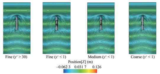
This section presents a qualitative analysis of the CFD results following the quantitative discussion in the previous section. Figure 13 displays the wave elevation contour from different CFD configurations at the same physical time (22.6 s) and scale (−0.062 3 m to 0.126 m). The impact of different y+ values on the fine configuration is evident from the figure. Despite a higher roll amplitude for y+ > 30, water on the deck did not appear. Conversely, water on the deck was observed when y to the plus less than 1 was used for the medium and coarse configurations. The viscous effect near the hull surface, particularly on the deck, was prominently noticeable between different y+ values.
Figure 14 illustrates the velocity magnitude of each configuration at the same physical time (22.6 s) and the same scale, ranging from 0 m/s to 0.5 m/s. It is evident that the total number of near-wall layers significantly impacts the velocity magnitude close to the hull. Specifically, for y+ < 1 with 12 layers, the velocity is smoothly captured, particularly near the bilge area. On the other hand, the thickness of the colour layer around the hull for y+ > 30 (single prism layer) is greater, dominated by a single value, and the degradation of velocity cannot be accurately captured despite using a logarithmic law region in that single near-wall layer.
When 12 prism layers were applied, the low velocity area near the no-slip boundary condition of the hull thins and exhibited a greater variation in velocity values. This means the different velocities around the hull can be captured well. The low y+ approach yields a better agreement with the experimental results, as shown in Table 8. Therefore, it is important to maintain y+ < 1 to produce the good result in the CFD simulation. To do this, Equation (16)‒(19) can be used to determine the desired y+. As explained earlier in Figure 2 (flow chart) in this study, this fine configuration was applied to other CFD simulations which are roll decay simulations to determine the ratio of linear roll damping and direct CFD simulations of small fishing boat on parametric roll.
5.2 Susceptibility assessment results
5.2.1 Roll damping results
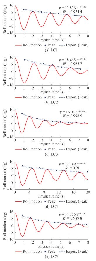
Figure 15 shows the result of roll decay simulations in each load case. The linear roll damping ratio (B/Bc), which is the ratio of roll damping to critical roll damping, was determined from the roll amplitude decrement. This can be described in the exponential equation (e−ζωnt), which is similar to μ in Equation (6). The term of μ in Equation (6) consists of ζωn, where ζ is the ratio between the linear roll damping and critical roll damping (B/Bc) and ωn is natural roll frequency in rad/s. Once μ is determined from the regression, which is shown in Figure 15, the ratio of linear roll damping, ζ can be determined by dividing μ by ωn.
The present study provides the linear roll damping ratio results in Table 10. To benchmark the numerical results, these values were compared with those obtained from the Ikeda's method, which is an empirical method provided in the ShipX software. As seen in Table 10, the comparison between the CFD and the Ikeda's method results shows a sufficient similarity, considering the approximate nature of the Ikeda's method.
Table 10 Comparison of the linear roll damping between the CFD and Ikeda's methodLoad case ShipX calculation (Ikeda's method) Roll damping ratio calculation CFD linear roll damping ratio Difference (%) Ixx (kg⋅m) Ixxadd (kg⋅m) B (kg⋅m/s) fn (1/s) Bc (kg⋅m/s) ζ (B/Bc) μ (Figure 15) ωn (rad/s) ζ (μ/ωn) 1 637.00 337.00 692.28 4.93 9 608.12 0.07 0.163 3.14 0.05 −27.8 2 1 160.00 441.00 1 064.80 4.93 15 793.23 0.07 0.253 3.14 0.08 20.1 3 509.00 441.00 1 067.30 6.17 11 729.14 0.09 0.433 3.93 0.11 20.9 4 2 130.00 456.00 1 241.10 2.26 11 698.79 0.11 0.056 1.44 0.04 −63.2 5 675.00 456.00 1 243.40 6.28 14 212.57 0.09 0.289 4.00 0.07 −17.7 The ratio of roll damping, ζ from ShipX, was calculated using the critical roll damping, Bc, which is defined as Bc = 2(Ixx + (Ixx)a) fn (kg⋅m/s), where Ixx is the moment of inertia of roll and (Ixx)a is added moment of inertia of roll, and fn is the natural roll frequency (1/s). Both moment of inertia values as well as the roll damping, B are taken from ShipX. As shown in Table 10, irrespective of the vertical load position, the roll damping, B, increased with displacement (LC1, LC2-LC3, and LC4-LC5).
However, the values of the linear roll damping ratio, ζ, varied for each load case, indicating that the vertical load position impacted the critical damping, Bc. As shown in Table 10, the moment of inertia of roll, Ixx, differed in each load case, while the added moment of inertia, (Ixx)a, was the same for the same displacement. This implies that the ratio of the linear roll damping, ζ, was affected by the different loading conditions, with the vertical load position playing a crucial role in this change. Unlike B and (Ixx)a, which are only influenced by displacement, the vertical loading position influenced the roll radius of gyration, kxx, resulting in varying values of the moment of inertia of roll, Ixx, even when the displacement was the same.
The ratio of roll damping value obtained from the CFD simulation was used to assess the susceptibility criteria of parametric roll according to ABS' rules (2019). If the ratio is unknown, the ABS guidelines recommend using the following range of roll damping ratios: μ = 0.03, 0.05, 0.075, 0.10. However, the values obtained from the roll decay CFD simulation in this paper were found to be better than using the range of μ recommended by ABS. The accuracy in determining this coefficient is important for assessing the susceptibility criteria, especially in criterion 2 (Eq. 10), where the effective roll damping is evaluated to determine whether it exceeds the threshold.
5.2.2 Susceptibility criteria assessment results
Table 11 shows the results of the susceptibility criteria analysis for the vessel. Criterion 1 is satisfied for all load cases, as shown in Figure 16, indicating that the vessel has the potential to experience parametric roll. However, the vessel's behaviour depends on the effective damping, as shown in Criterion 2. If the effective damping is lower than the damping threshold (Equation (10) is satisfied), then parametric roll is expected to occur.
Table 11 The results of the Susceptibility CriteriaLoad case Criterion 1 Criterion 2 p q Eq. 9 Effective damping Damping threshold Eq. 10 1 0.249 0.078 Satisfied 0.025 0.079 Satisfied 2 0.248 0.051 Satisfied 0.049 0.052 Satisfied 3 0.247 0.028 Satisfied 0.061 0.028 Not satisfied 4 0.249 0.063 Satisfied 0.017 0.064 Satisfied 5 0.249 0.015 Satisfied 0.037 0.015 Not satisfied Referring to the Susceptibility Criteria in Table 11, load cases 3 and 5 have a higher effective damping roll than the damping threshold, which means that the parametric roll is not expected to occur in these load cases. Other load cases (LC1, LC2, ands LC4) are predicted to experience parametric roll because Criterion 2 was satisfied. In these conditions the damping roll in each load case is lower than that damping threshold. Because the roll damping is below the threshold, the roll damping is not high enough to reduce the roll motions significantly caused by the periodic variation of the restoring roll moment.
The prediction of PR occurrence in the early stage has been carried out by using two different methods. First, level 1 assessment of PR from Second Generation of Intact Stability IMO and second, the Susceptibility Criteria of Parametric Roll from ABS. Both assessment methods give the same results, whereas LC3 and LC5 do not result in parametric roll. Nevertheless, the amplitude of parametric roll of suspected load case is still to be confirmed by carrying out the CFD simulations. The following sub-section will discuss the results of direct CFD simulation of PR for the small fishing vessel.
5.3 CFD results of PR simulation of fishing boats
5.3.1 Results of averaged y+
Figure 17 shows the results of averaged y+ on the wetted surface area for all load cases. As can be seen in the figure that all averaged y+ are below 1. The determination of the total number of layers from Equation (19) was successful in achieving the targeted y+ value (ytarget+ = 0.7) which was also used when studying the KCS hull performance. This is used as an indication that the velocity gradient near the wall is captured.
The determination of the total number of layers for all load cases (except LC4) used the highest speed only (speed for LC3) and resulted in 17 layers. Then, with the same total number of layers, the averaged y+ in each load case are varying because the different speeds result in different y+. The lower speeds resulted in the lower averaged y+. Nevertheless, the average values are always y+ < 1.
5.3.2 Parametric roll amplitude
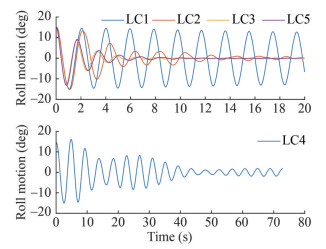
Figure 18 presents the outcomes of CFD modelling for the various load cases (LC1 to LC5) under a presumed state of parametric roll. To hasten the occurrence of the roll phenomenon, the vessel was initially inclined at 15° and sailed under specific wave and velocity conditions as detailed in Table 4. It should be noted that the initial roll angle did not impact the obtained parametric roll amplitude results, as reported by (Liu et al., 2021).
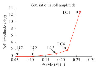
It is evident that LC3 and LC5 did not undergo parametric roll, as evidenced by the level 1 SGIS results in Table 5 and the susceptibility criteria presented in Table 11. The roll amplitude in these cases decreased rapidly and dissipated after 10 s of physical time. By contrast, for LC2 and LC4, parametric roll persisted with a small amplitude. Initially, after the boat was tilted 15°, there was some parametric roll with higher amplitude than in the previous cycles. However, once the roll amplitude became steady, LC2 did not exhibit parametric roll, while LC4 did. The highest roll amplitude was observed in LC1. After the boat was released, the roll amplitude of LC1 decreased very slowly, indicating that the roll amplitude did not differ significantly from the initial values.
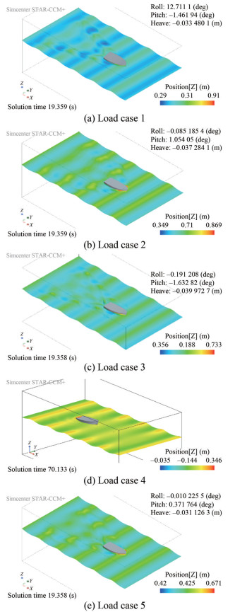
Figure 19 shows the contour of wave elevation based on CFD simulations. It can be seen that the produced wave from inlet boundary was created well. Also, close to the left and the right-side extents of the computational domain and the outlet boundaries, it can be seen that there are no reflection waves that can disturb the boat response. These conditions are caused by implementing the forcing method close to those boundaries as mentioned in subsection 4.5.6.
FFT analysis was used to define the roll amplitude for each load case. It should be noted that the last three cycles from the roll amplitude were used to transform the time domain into the frequency domain. Following this sub-section, the last three cycles of other degrees of freedom, such as pitch and heave were also used to quantify the performance of the vessel. The results of these analyses were compared to the roll motion to investigate the impact of parametric roll on other aspects of the vessel's behaviour.
5.3.3 Roll, pitch, and heave motions
The present study utilised a coordinate system described in section 4.5.4, where the X-direction coincides with the length of the boat. A positive X-direction represents the direction towards the bow. With regards to rotational motion, the positive value is equivalent to a clockwise direction. For X-direction rotational motion (roll motion), a positive value indicates that the boat is rolling towards the starboard side. Conversely, in the case of pitch motion, a positive Y-direction represents the direction towards the port side, and a negative Y-direction represents the starboard side. Thus, when the boat rotates in a positive Y-direction, it will pitch downwards from the bow.
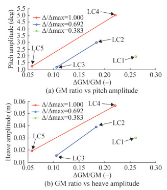
The results of the FFT analysis of roll, pitch, and heave amplitude are shown in Table 12. Referring to Equation (20), the FFT results consist of φ0 and φn, which are the average (mean) and the amplitude. Based on the results, it can be inferred that the largest parametric roll amplitude occurs in LC1, which is 12.755 6°. The second one is LC4 which has a roll amplitude of 1.837 6°. The other load cases are considered to have no parametric roll, as their roll amplitude is close to 0°.
Table 12 FFT results of roll, pitch, and heave motionsLoad case Roll (°) Pitch (°) Heave (m) Mean Amplitude Mean Amplitude Mean Amplitude 1 −0.116 44 12.755 6 −3.053 6 1.945 8 −0.017 479 0.029 679 2 0.152 17 0.775 6 −1.501 8 2.996 8 −0.007 56 0.038 771 3 −0.094 458 0.031 794 −2.667 7 1.156 9 −0.038 993 0.014 939 4 −0.022 276 1.837 6 −0.982 83 5.039 5 −0.009 716 5 0.056 559 5 −0.063 592 0.024 213 −0.701 97 1.230 5 −0.021 113 0.018 813 In general, among the five load cases, only LC1 can be considered dangerous due to the occurrence of parametric roll. Table 4 indicates that all load cases are simulated with similar relative wave conditions, and that the speeds for LC1, LC3, and LC5 are also similar at around 2 m/s. Despite these similarities, there are differences in the roll motion response among these load cases. Specifically, LC1 shows a considerable roll amplitude, while LC3 and LC5 do not. This implies that the different loading conditions are sensitive to the parametric roll behaviour.
Based on Table 12, there is no correlation between the amplitude of roll to the pitch motion. The highest roll amplitude (LC1) has the lowest pitch motion amplitude (1.94°), while LC4 results in a pitch angle of 5.04°. This shows no correlation between roll and pitch motion amplitudes when the boat moves in head waves. The roll-heave correlation is similar to the roll-pitch correlation. It can also be seen in Table 12 that the order from the highest to the lowest for heave motions is the same as for pitch motions. LC4, which results in the highest heave motions, also results in the highest pitch motions and so for the lowest heave and pitch that were occurred on LC3.
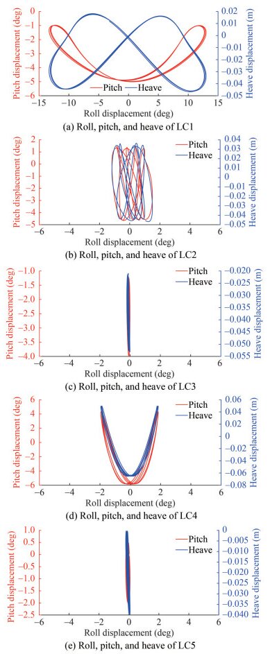
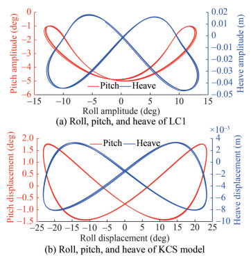
The correlations between roll, and pitch/heave motions during parametric roll phenomenon can be explained by examining the cycles of each mode of motion. Specifically, pitch and heave motions complete two cycles for each roll cycle. The total number of cycles roll, and pitch/heave can then be used to establish their relationship. Figure 20 shows that parametric roll occurs when the total cycle of pitch/heave is approximately twice that of roll.
Figure 20 illustrates a comparison between the motion of roll-pitch and roll-heave for LC1 to LC5. The graph presents a vertical line for the load cases, such as LC3, LC5, and LC2, where the boat did not experience parametric roll. In contrast, for LC1 and LC4, which experienced the parametric roll, it can be observed that pitch and heave underwent two cycles during one cycle of roll motion. This is a typical feature of parametric roll, where the encounter wave period is twice as roll natural period. Heave and pitch have the same period as the encounter waves in head waves.
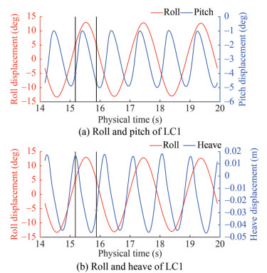
Examining Figure 20 for LC1, it can be seen that with the same roll angle, there are two different displacement values for both heave and pitch, but this does not mean that the boat experienced two different heave and pitch displacements simultaneously. It should be noted that Figure 20 only compares the displacement behaviour between roll-pitch and roll-heave and the figure is not time-dependent. This can be explained well in Figure 21 when the time series of roll-pitch and roll-heave of LC1 are shown.
Based on Figure 21, it is clearly shown that with the same roll angle (5°), the displacement of heave and pitch are different because there is a different physical time in the same roll angle (5°). Each physical time has a different displacement for both heave and pitch.
Figure 22 shows the phase portrait of the roll, pitch, and heave motion between LC1 and the KCS model, which serves as the verification study. Both conditions demonstrate the parametric roll phenomenon, with two cycles of pitch and heave in each cycle of the roll. The heave motion of LC1 and KCS model attain their highest and lowest values at half and maximum roll. For example, LC 1's highest and lowest heave occurred at a roll of around 6° and 12°, respectively. In comparison, the KCS model's highest and lowest heave occurred at a roll of approximately 12° and 24°, respectively. However, the pattern for the pitch motion is different. The KCS model follows the same pattern as the heave motion for the maximum and minimum pitch. In contrast, the fishing boat exhibits a distinct minimum pitch pattern, which appears at a roll of less than about 6°.
5.4 The influence of loading condition
Changes in the loading condition of a fishing vessel often occur during operation. As discussed in the background section, various factors can affect parametric rolling, including GM Ratio and flare shape. The subsequent subsection investigates the extent to which changes in loading condition impact GM Ratio and flare shape, ultimately affecting seakeeping and parametric rolling behaviour.
5.4.1 Flare distribution
The GM Ratio is also influenced by the stern shape and the flare of stern and bow, as stated by Neves et al. (1999) and France et al (2003). Different loading conditions applied to a certain ship will result in a change in the draught of the boat. Thus, the submerged hull shape also changes significantly, especially for the V-shape hull, which is mostly common in fishing boats. This condition makes a different longitudinal distribution of half breadth (Y) and flare (dY/dZ) at the water line, as shown in Figure 23.
Figure 23 describes the longitudinal distribution of the half breadth and flare at the water line for LC1 and LC5. LC1 is the lightest weight and has the highest parametric roll amplitude. Conversely, LC5 is the heaviest and has no parametric roll. Based on the figure, the half breadth distribution for both load cases is entirely different. Moreover, the V-shaped of hull form results in a significant change in flare distribution because of the low draught due to low displacement. As can be seen from Figure 23, the longitudinal position of LC1 is characterised by a flare (dY/dZ) of more than 1. Unlike LC5, which only has a flare of more than 1 at X/Lbp 0.6‒0.85.
As stated by Neves et al. (1999), the significant difference in the longitudinal distribution of flare influences the parametric roll amplitude. Furthermore, France et al. (2003) clarified this influence by comparing the flare angle from one station in the bow started from 0° to 40°. The value of 0° which means when there is no flare curve there is no PR, while the flare angle of 40° results in the highest PR amplitude. The results clearly explain that the hull shape above the water line significantly influences the PR. When the vessel is pitching and heaving, the high flare angle changes the buoyancy compared to the straight case which results in a GM variation.
5.4.2 GM Ratio
Figure 24 depicts the influence of displacement change on the KM value. The lowest displacement corresponds to LC1, which indicates 0% fish tank capacity. Subsequently, the displacement increases to 50% fish tank capacity for LC2 and LC3, and full load condition for LC4 and LC5. The graph illustrates a decreasing trend of KM with increasing displacement. LC1 exhibits a GM/KM ratio of more than 0.4, while LC2 and LC3 are approximately 0.4 and 0.6, respectively. LC4 and LC5 show a GM/KM ratio of less than 0.2 and 0.6, respectively.
Based on Figure 24, it can be seen that the actual GM between LC1, LC3, and LC5 are relatively similar, but they are characterised by a different GM/KM ratio. The higher displacement cases have the higher GM/KM ratios. Following this, the GM Ratio (ΔGM/GMcalm), which is known as level 1 assessment of PR, was calculated from the combination of GM/KM ratios and displacement change (relative to the maximum displacement) to observe the influence of the loading conditions. The impact of changes in both the vertical loading position (GM/KM ratio) and displacement on GM Ratio is illustrated in Figure 25.
Figure 25 illustrates the impact of different loading conditions on GM Ratio in head waves with a wavelength of λ = 5.0 m and a wave height of Hw = 0.3 m. GM Ratio is a Level 1 assessment of parametric roll in the Second Generation of Intact Stability (SGIS) as described in Equation (2). The ratio of displacement to the maximum displacement represents the change in displacement, and the GM/KM ratio represents the change in vertical loading condition. The GM Ratio threshold (Rpr) for the ship without a bilge keel is 0.17. The figure also shows the GM Ratios for all load cases, which are taken from Table 5.
The trend in Figure 24 shows that at the same GM/KM ratio, the lowest displacement has the highest GM Ratio. On the other hand, observing each displacement, the lower GM/KM ratio, the higher GM Ratio. Referring to Table 2 (loading condition) and Figure 23 (KM and GM), the GM for LC1 and LC5 are quite similar (0.763 m and 0.657 m), but both GM Ratio results are different, as both GM/KM ratios are different. This indicates that the GM/KM ratio is more essential than the actual GM. The KM for each load case should be considered as well in a parametric roll.
5.4.3 Relationship between GM ratio to the amplitude of roll, pitch and heave
When the GM Ratio is linked to the parametric roll amplitude, it may be concluded that a higher the GM Ratio is associated with a greater roll amplitude, as depicted in Figure 26. The aforementioned figure indicates that the roll amplitude commences to escalate when the GM Ratio surpasses the threshold of 0.17, which is attributed to LC2, LC4, and LC1. This discovery aligns with SGIS's evaluation of parametric roll, which necessitates identifying the roll motion amplitude in the event of level 1 failure (i.e., GM Ratio exceeding the threshold) and proceeding to level 2 or direct stability analysis.
The present investigation examines not only LC3 and LC5, which passed level 1 SGIS assessment for Parametric Roll, but also other load cases that failed, by utilizing fully nonlinear URANS CFD simulation to assess their parametric roll amplitudes. Of all the load cases considered, LC1, which has the lowest weight, poses the greatest danger to fishing boats due to its elevated parametric roll amplitude. As displacement and GM/KM ratio increase, the GM Ratio decreases, leading to a reduction in parametric roll amplitude. Regardless of the boat's speed or wave direction, the operator should not run the vessel with an empty load and should lower the vertical load's position to prevent parametric roll from occurring during operation.
In our previous study (Iqbal et al., 2023), the heave, pitch, and roll motions of the same fishing vessel modelled herein were predicted by using the linear strip theory. Based on our findings, both vertical load position and displacement change the roll motions. The roll natural frequency as well as roll damping are changed when the displacement and GM are altered. On the other hand, pitch and heave motions were not influenced by the vertical loading condition, which only changed when the displacement was varied. Based on this, the influence of GM Ratio on the pitch and roll amplitude can be observed with the same displacement.
Figure 27 shows the correlation between GM Ratios and the pitch and heave amplitudes. The figure elucidates why there exists a discrepancy between the amplitude of roll and pitch and heave, as discussed in Section 5.3. A higher roll amplitude does not necessarily entail that pitch and heave amplitudes are also high. In fact, with the same displacement, variations in GM play a significant role in increasing pitch and heave amplitudes.
The red line in Figure 27 is the full load displacement, consisting of LC4 and LC5. As the GM Ratio increases, the amplitude of pitch increases from 1.23° to 5.03°. This change was replicated in LC 2 and LC3, where the fish tank capacity was 50% full. It can be seen that the pitch amplitudes increased from 1.15° to 2.99° in these cases. As there is no vertical loading position change in LC1, it is not possible to observe the influence of GM Ratio on the pitch and heave amplitudes. However, based on two different displacements, both amplitudes will increase if the GM increases. All trends observed for pitch were similar in the case of heave.
The above findings show that the parametric roll amplitudes do not influence the pitch and heave amplitudes. The GM Ratio, which is the level 1 assessment of SGIS form IMO, is the only one that affects the amplitude of roll, pitch, and heave. In this paper, the GM Ratio was determined from different loading conditions, which are the vertical load position (GM/KM) and displacement (Δ/Δmax). Both of these parameters change the amplitudes of parametric roll. On the other hand, the influence of GM Ratio on the amplitudes of pitch and roll can be observed with the same displacement. This means, the GM Ratios that change the amplitudes of pitch and heave motions are based on vertical load position only.
The level 1 assessment of SGIS from IMO is a reliable tool to detect the parametric roll in the early design stages. Through the utilisation of fully nonlinear Computational Fluid Dynamics (CFD) simulation, this current study elucidated how the pitch and heave amplitudes are influenced by the independent increase of GM Ratio, regardless of the roll amplitude. This research imparts vital information to the ship operator, specifically, the significance of maintaining the GM Ratio below the predetermined threshold, set at 0.17. To meet this criterion, the placement of the fish tank should be as low as possible to ensure a high GM/KM, and the vessel should be laden as heavily as possible by avoiding an empty fish tank.
6 Conclusions
Parametric roll simulations for the KCS model and a small fishing boat were carried out using a commercially available URANS solver. The result from fine configuration of mesh and time step was 3.66% lower compared to the available experimental test. The Grid Convergence Index showed an acceptable level of discretisation uncertainty of 2.76%. It was demonstrated that keeping the y+ value below unity is important to ensure the effect of viscous damping on the amplitudes of parametric roll is modelled accurately. The results showed that the fine configuration with the high y+ (30‒100) resulted in high roll amplitudes, overestimating the experimental results taken from the open literature by 16.33%.
Two assessments to detect the parametric roll occurrences in early design stages were carried out by using the level 1 assessment of Parametric roll on Second Generation of Intact Stability from IMO and the Susceptibility criteria of Parametric roll from ABS. Both returned the same results, where LC1, LC2, and LC 4 are predicted to exhibit parametric roll. The susceptibility criteria from ABS were also used to determine the design wave and vessel speed that was suspected to trigger parametric roll, which is useful in reducing the total number of CFD simulations.
Level 1 assessment is based on GM Ratios, while the susceptibility criteria is based on the frequency condition and the ratio of linear roll damping (B/Bc). With the damping threshold, the last criterion from ABS revealed that if the effective roll damping was sufficient the parametric roll motions were going to be very low. However, the accurate prediction of roll damping is necessary. To achieve this, the low speed CFD roll decay simulations in head waves were carried out.
Linear roll damping ratios obtained from CFD simulations were compared with those obtained from Ikeda's method using the ShipX software. It was revealed that the displacement of the vessel influenced the roll damping coefficient and added roll moment of inertia. Meanwhile, the displacement and vertical load position influenced the roll moment of inertia. All of these change the linear roll damping ratio. Even though the prediction of PR occurrence in the early stage has been carried out using two different methods, the amplitude of parametric roll of suspected load case still needs to be confirmed through the CFD simulations.
Based on the CFD simulations, LC1, surprisingly was the load case that had the highest parametric roll amplitude (12.76°) followed by LC4 (1.84°) and LC2 (0.78°). Meanwhile, LC3 and LC5, as predicted, did not result in parametric roll. It was also revealed that the parametric roll amplitude did not directly influence the amplitude of pitch and heave motions. A higher parametric roll amplitude does not indicate high pitch and heave amplitudes. The changes in loading conditions during operation also changed the longitudinal distribution of flare shape at the water line. The flare shape contributed to the occurrence of parametric roll, as it can significantly change the buoyancy as well as the GM when the boat is pitching and heaving in waves.
The GM Ratio (level 1 assessment of PR on SGIS from IMO) had a crucial role in changing the amplitudes of parametric roll, pitch, and heave. The roll amplitudes were increased when the GM Ratio caused by vertical load position (GM/KM) and displacement (Δ/Δmax) increased. With the same displacement, the amplitude of pitch and heave motions will also increase when the GM Ratio increased due to the change of vertical load position (GM/KM).
This research gives the information to the ship operator that it is important to keep the GM Ratio of the boat below the threshold, which is, in this case 0.17, to avoid the parametric roll occurrence and increase in pitch and heave motions during its operation. This can be achieved by placing the fish as low as possible (making the GM/KM high) and keeping the boat as heavy as possible (making the displacement high) by not keeping the fish tank empty.
Future work should focus on minimising power requirements while considering the boat's loading condition, as larger displacements can be used to avoid parametric roll occurrence. Still, it may result in higher resistance in calm water and waves. Additionally, as the boat operates at high Froude numbers, it may enter the displacement and semi-planning modes of motion.
Acknowledgement: Results were obtained using the ARCHIE-WeSt High-Performance Computer (www. archie-west. ac. uk) based at the University of Strathclyde. The work published in this paper is drawn from the first author's PhD thesis. The first author gratefully acknowledges Diponegoro University in Indonesia for giving a PhD scholarship to support his study at the University of Strathclyde, Glasgow.Competing interest The authors have no competing interests to declare that are relevant to the content of this article. -
Figure 1 Body plan of the research object (Liu et al., 2019)
Table 1 Main dimensions of the fishing boat (Tezdogan et al., 2018)
Parameter Value Length between perpendicular, LBP (m) 5.000 Breadth at the water line, B (m) 1.934 Depth to 1st deck, D (m) 1.196 Loaded draft, T (m) 0.350 Displacement, Δ(t) 1.858 Block coefficient, Cb 0.537 Mid-boat section coefficient, Cm 0.764 Wetted surface area, Aw (m2) 10.201 Maximum Froude number, Fr 0.590 Table 2 Loading condition of the fishing vessel operation (Iqbal et al., 2023)
Load case Description Ship weight (kg) LCG (m) KG (m) GM (m) 1 Empty load of fish 712.00 1.550 0.844 0.763 2 Half load of fish, upper deck 1 285.00 1.751 0.914 0.456 3 Half load of fish, below deck 1 285.00 1.751 0.557 0.813 4 Full load of fish, upper deck 1 858.00 1.828 1.064 0.163 5 Full load of fish, below deck 1 858.00 1.828 0.57 0.657 Table 3 Wave height information according to the Wave Scatter Data from IACS Recommendation
Wavelength, λ (m) Wave height, Hw (m) Hw/λ 50 5.9 0.12 100 11.6 0.12 150 14.2 0.09 200 15.1 0.08 250 15.2 0.06 300 14.6 0.05 350 13.6 0.04 400 12.0 0.03 450 9.9 0.02 Table 4 Result of vessel speed and wave direction for λ = 5.0 m and Hw = 0.3 m based on Eq. 1
Load case Tn(s) Boat speed, VPR (m/s) Wave direction Te (s) Te/Tn 1 2.00 2.37 Head waves (2ωm > ωw) 0.968 0.48 2 2.00 1.33 Head waves (2ωm > ωw) 1.212 0.61 3 1.60 2.85 Head waves (2ωm > ωw) 0.886 0.55 4 4.38 0.35 Following waves (2ωm < ωw) 2.046 0.47 5 1.57 2.36 Head waves (2ωm > ωw) 0.970 0.62 Table 5 The results of Level 1 SGIS (Eq. 2)
Load case ΔGM GMcalm ΔGM/GMcalm RPR Status 1 0.419 0.763 0.261 0.17 Failed 2 0.252 0.456 0.184 0.17 Failed 3 0.145 0.813 0.106 0.17 Pass 4 0.271 0.163 0.221 0.17 Failed 5 0.071 0.657 0.058 0.17 Pass Table 6 Computational domain size of similar previous studies
Reference Upstream Downstream Top Bottom Transverse (Sadat-Hosseini et al., 2010) 0.5L 2.0L 0.25L 1.0L 1.0L (Ma et al., 2018) 2.0λ 4.5λ 1.5λ 2.5λ 2.5λ (Liu et al., 2021) 1.0L 3.0L 0.4L 1.0L 1.0L 7(a) Main dimensions of the KCS model (1:100)
Parameters Value Length between perpendicular, Lbp (m) 2.3 Breadth at water line, B (m) 0.322 Depth, D (m) 0.19 Loaded draft, T (m) 0.108 Displacement (kg) 52.31 Longitudinal centre of buoyancy, LCB from AP (m) 1.116 Height of centre of gravity, KG (m) 0.136 6 Metacentric height, GM (m) 0.012 7 0.324 2, Kxx/B, Kyy/Lbp, Kzz/Lbp 0.249 5, 0.246 5 Roll natural period, Tn (s) 2.16 7(b) Simulation conditions
Parameters Value V (m/s) 0.40 Wavelength, λ/Lbp 1.00 Wave height/wavelength, Hw/λ 0.02 Te/Tn 0.464 Table 8 Comparison of roll amplitude for different y+ values
Parametric roll results y+ > 30 y+ < 1 CFD (°) 28.77 23.77 EFD (°) (Yu et al., 2018; 2019) 24.68 24.68 Error (%) 16.33 -3.66 Table 9 Verification results
Parameter Value Fine configuration, N1 Total mesh = 13 305 894;
Time step = 0.005 000Medium configuration, N2 Total mesh = 8 479 668;
Time step = 0.006 150Coarse configuration, N3 Total mesh = 5 544 893;
Time step = 0.007 626Refinement ratio, r21 1.23 Refinement ratio, r32 1.24 Fine solution, S1(°) 23.769 8 Medium solution, S2(°) 23.120 6 Coarse solution, S3(°) 21.584 3 Medium-fine, ɛ21(°) −0.649 2 Coarse-medium, ɛ32(°) −1.536 3 Convergence ratio, R 0.422 6 (Monotonic, 0 < R < 1) Order of accuracy, p 3.889 3 GCI (%) 2.76 Table 10 Comparison of the linear roll damping between the CFD and Ikeda's method
Load case ShipX calculation (Ikeda's method) Roll damping ratio calculation CFD linear roll damping ratio Difference (%) Ixx (kg⋅m) Ixxadd (kg⋅m) B (kg⋅m/s) fn (1/s) Bc (kg⋅m/s) ζ (B/Bc) μ (Figure 15) ωn (rad/s) ζ (μ/ωn) 1 637.00 337.00 692.28 4.93 9 608.12 0.07 0.163 3.14 0.05 −27.8 2 1 160.00 441.00 1 064.80 4.93 15 793.23 0.07 0.253 3.14 0.08 20.1 3 509.00 441.00 1 067.30 6.17 11 729.14 0.09 0.433 3.93 0.11 20.9 4 2 130.00 456.00 1 241.10 2.26 11 698.79 0.11 0.056 1.44 0.04 −63.2 5 675.00 456.00 1 243.40 6.28 14 212.57 0.09 0.289 4.00 0.07 −17.7 Table 11 The results of the Susceptibility Criteria
Load case Criterion 1 Criterion 2 p q Eq. 9 Effective damping Damping threshold Eq. 10 1 0.249 0.078 Satisfied 0.025 0.079 Satisfied 2 0.248 0.051 Satisfied 0.049 0.052 Satisfied 3 0.247 0.028 Satisfied 0.061 0.028 Not satisfied 4 0.249 0.063 Satisfied 0.017 0.064 Satisfied 5 0.249 0.015 Satisfied 0.037 0.015 Not satisfied Table 12 FFT results of roll, pitch, and heave motions
Load case Roll (°) Pitch (°) Heave (m) Mean Amplitude Mean Amplitude Mean Amplitude 1 −0.116 44 12.755 6 −3.053 6 1.945 8 −0.017 479 0.029 679 2 0.152 17 0.775 6 −1.501 8 2.996 8 −0.007 56 0.038 771 3 −0.094 458 0.031 794 −2.667 7 1.156 9 −0.038 993 0.014 939 4 −0.022 276 1.837 6 −0.982 83 5.039 5 −0.009 716 5 0.056 559 5 −0.063 592 0.024 213 −0.701 97 1.230 5 −0.021 113 0.018 813 -
American Bureau of Shipping (ABS) (2019) Guide for the Assessment of Parametric Roll Resonance in the Design of Container Carriers Burmester S, Vaz G, el Moctar O (2020) Towards credible CFD simulations for floating offshore wind turbines. Ocean Engineering, 209: 107237. https://doi.org/10.1016/j.oceaneng.2020.107237 Celik IB, Ghia U, Roache PJ, Freitas CJ (2008) Procedure for estimation and reporting of uncertainty due to discretization in CFD applications. Journal of Fluids Engineering, 130(7): 078001. https://doi.org/10.1115/1.2960953 France WN, Levadou M, Treakle TW, Paulling JR, Michel RK, Moore C (2003) An investigation of head-sea parametric rolling and its influence on container lashing systems. Marine Technology and SNAME News, 40(1): 1-19. https://doi.org/10.5957/mt1.2003.40.1.1 Francescutto A (2001) An experimental investigation of parametric rolling in head waves. Journal of Offshore Mechanics and Arctic Engineering, 123(2): 65-69. https://doi.org/10.1115/1.1355247 Galbraith A, Boulougouris E (2015) Parametric rolling of the tumblehome hull using CFD. In Proceedings of the 12th International Conference on the Stability of Ships and Ocean Vehicles, 535-543 Ghamari I, Faltinsen OM, Greco M, Lugni C (2017) Parametric resonance of a fishing vessel with and without anti-roll tank: an experimental and numerical study. in Volume 7A: Ocean Engineering. American Society of Mechanical Engineers, V07AT06A012. https://doi.org/10.1115/OMAE2017-62053 Ghamari I, Greco M, Faltinsen OM, Lugni C (2020) Numerical and experimental study on the parametric roll resonance for a fishing vessel with and without forward speed. Applied Ocean Research, 101: 102272. https://doi.org/10.1016/j.apor.2020.102272 Hashimoto H, Furusho K (2022) Influence of sea areas and season in navigation on the ship vulnerability to the parametric rolling failure mode. Ocean Engineering, 266: 112714. https://doi.org/10.1016/j.oceaneng.2022.112714 Himeno Y (1981) Prediction of ship roll damping-state of the art. The University of Michigan, College of Engineering, Department of Naval Architecture and Marine Engineering. Report No. 239 [Preprint] Hirt CW, Nichols BD (1981) Volume of fluid (VOF) method for the dynamics of free boundaries. Journal of Computational Physics, 39(1): 201-225 https://doi.org/10.1016/0021-9991(81)90145-5 Hooft JP (1987) Mathematical description of the manoeuvrability of high-speed surface ships Hosseini SHS (2009) CFD prediction of ship capsize: parametric rolling, broaching, surf-riding, and periodic motions. The University of Iowa Ikeda Y (1979) On roll damping force of ship-effect of hull surface pressure created by bilge keels. University of Osaka Prefacture, Department of Naval Architecture, Japan, Report No. 00402. Journal of Society of Naval Architects of Japan, 165 [Preprint] Ikeda Y, Himeno Y, Tanaka N (1977) On eddy making component of roll damping force on naked hull. Journal of the society of Naval Architects of Japan, 1977(142): 54-64 https://doi.org/10.2534/jjasnaoe1968.1977.142_54 IMO (2008) International Code of Intact Stability. London, UK Iqbal M, Terziev M, Tezdogan T, Incecik A (2023) Operability analysis of traditional small fishing boats in Indonesia with different loading conditions. Ships and Offshore Structures, 18(7): 1060-1079. https://doi.org/10.1080/17445302.2022.2107300 ITTC I (2011) Practical guidelines for ship CFD applications. Recommended Procedures and Guidelines, 18 Kato H (1957) On the frictional resistance to the rolling of ships. Journal of Zosen Kiokai, 1957(102): 115-122 https://doi.org/10.2534/jjasnaoe1952.1957.102_115 Lin WM, Salvesen N (1997) Nine years of progress with LAMP-the large amplitude motion program. Science Applications International Corp Report SAIC-97/1079 [Preprint] Liu L, Chen M, Wang X, Zhang Z, Yu J, Feng D (2021) CFD prediction of full-scale ship parametric roll in head wave. Ocean Engineering, 233: 109180. https://doi.org/10.1016/j.oceaneng.2021.109180 Liu L, Feng D, Wang X, Zhang Z, Yu J, Chen M (2022) Numerical study on the effect of sloshing on ship parametric roll. Ocean Engineering, 247: 110612. https://doi.org/10.1016/j.oceaneng.2022.110612 Liu W, Demirel YK, Djatmiko EB, Nugroho S, Tezdogan T, Kurt RE, Supomo H, Baihaqi I, Yuan Z, Incecik, A. (2019) Bilge keel design for the traditional fishing boats of Indonesia's East Java. International Journal of Naval Architecture and Ocean Engineering, 11(1): 380-395. https://doi.org/10.1016/j.ijnaoe.2018.07.004 Liu Y, Liu L, Maki A, Bu S, Dostal L (2023) Research on second level of vulnerability criteria of parametric rolling with stochastic stability theory. Ocean Engineering, 284: 115043. https://doi.org/10.1016/j.oceaneng.2023.115043 Lu J, Gu M, Umeda N (2016) A study on the effect of parametric roll on added resistance in regular head seas. Ocean Engineering, 122: 288-292. https://doi.org/10.1016/j.oceaneng.2016.06.016 Ma S, Ge W, Ertekin RC, He Q, Duan W (2018) Experimental and numerical investigations of ship parametric rolling in regular head waves. China Ocean Engineering, 32(4): 431-442. https://doi.org/10.1007/s13344-018-0045-6 Maruo H (1963) Resistance in waves, research on seakeeping qualities of ships in Japan. The Society of Naval Architects of Japan, 8: 67-102 Maruyama Y, Maki A, Dostal L, Umeda N (2023) Estimation of acceleration probability density function for parametric rolling using PLIM', Ocean Engineering, 280: 114561. https://doi.org/10.1016/j.oceaneng.2023.114561 Menter FR (1994) Two-equation eddy-viscosity turbulence models for engineering applications. AIAA Journal, 32(8): 1598-1605. https://doi.org/10.2514/3.12149 Miller ER (1974) Roll Damping Muzaferija S (1998) Computation of free surface flows using interface-tracking and interface-capturing methods. Nonlinear water-wave interaction. Computational Mechanics, Southampton [Preprint] Neves MAS (2002) Experimental analysis on parametric resonance for two fishing vessels in head seas. In Proceedings of the 6th International Ship Stability Workshop. Webb Institute, P2002-1 Neves MAS (2011) An investigation on head-sea parametric rolling for two fishing vessels. In Contemporary Ideas on Ship Stability and Capsizing in Waves. Springer, 231-252 Neves MAS, Pérez NA, Valerio L (1999) Stability of small fishing vessels in longitudinal waves. Ocean Engineering, 26(12): 1389-1419. https://doi.org/10.1016/S0029-8018(98)00023-7 Neves MAS, Rodríguez CA (2006) On unstable ship motions resulting from strong non-linear coupling. Ocean Engineering, 33(14-15): 1853-1883. https://doi.org/10.1016/j.oceaneng.2005.11.009 Park DM, Kim Y, Song KH (2013) Sensitivity in numerical analysis of parametric roll. Ocean Engineering, 67: 1-12. https://doi.org/10.1016/j.oceaneng.2013.04.008 Paulling JR, Rosenberg RM (1959) On unstable ship motions resulting from nonlinear coupling. Journal of Ship Research, 3(2): 36-46. https://doi.org/10.5957/jsr.1959.3.2.36 Ravenna R, Song S, Shi W, Sant T, De Marco Muscat-Fenech C, Tezdogan T, Demirel YK (2022) CFD analysis of the effect of heterogeneous hull roughness on ship resistance. Ocean Engineering, 258: 111733. https://doi.org/10.1016/j.oceaneng.2022.111733 Riberio e Silva S, Turk A, Guedes Soares C, Prpić-Oršić J (2010) On the parametric rolling of container vessels. Brodogradnja: Teorija i praksa brodogradnje i pomorske tehnike, 61(4): 347-358 Richardson LF (1911) The approximate arithmetical solution by finite differences of physical problems involving differential equations, with an application to the stresses in a masonry dam', Philosophical Transactions of the Royal Society of London. Series A, Containing Papers of a Mathematical or Physical Character, 210(459-470): 307-357. https://doi.org/10.1098/rsta.1911.0009 Rodríguez CA, Ramos IS, Esperança PTT, Oliveira, MC (2020) Realistic estimation of roll damping coefficients in waves based on model tests and numerical simulations. Ocean Engineering, 213: 107664. https://doi.org/10.1016/j.oceaneng.2020.107664 Sadat-Hosseini H, Stern F, Olivieri A, Campana EF, Hashimoto H, Umeda N, Bulian G, Francescutto A (2010) Head-wave parametric rolling of a surface combatant', Ocean Engineering, 37(10): 859-878. https://doi.org/10.1016/j.oceaneng.2010.02.010 Schumacher A, Ribeiro e Silva S, Guedes Soares C (2016) Experimental and numerical study of a containership under parametric rolling conditions in waves. Ocean Engineering, 124: 385-403. https://doi.org/10.1016/j.oceaneng.2016.07.034 Siemens (2022) Star-CCM+ User Guide version 17.02 Spanos D, Papanikolaou A (2006) Numerical simulation of a fishing vessel in parametric roll in head seas. Marine Systems & Ocean Technology, 2(1-2): 39-44. https://doi.org/10.1007/BF03449182 Spanos D, Papanikolaou A (2007) Numerical simulation of parametric roll in head seas. International Shipbuilding Progress, 54(4): 249-267 Terziev M, Tezdogan T, Incecik A (2022) Scale effects and full-scale ship hydrodynamics: A review. Ocean Engineering, 245: 110496. https://doi.org/10.1016/j.oceaneng.2021.110496 Tezdogan T, Shenglong Z, Demirel YK, Liu W, Leping X, Yuyang L, Kurt RE, Djatmiko EB, Incecik, A (2018) An investigation into fishing boat optimisation using a hybrid algorithm. Ocean Engineering, 167: 204-220. https://doi.org/10.1016/j.oceaneng.2018.08.059 Wackers J, Koren B, Raven HC, van der Ploeg A, Starke AR, Deng GB, Queutey P, Visonneau M, Hino T, Ohashi K (2011) Free-surface viscous flow solution methods for ship hydrodynamics. Archives of Computational Methods in Engineering, 18(1): 1-41. https://doi.org/10.1007/s11831-011-9059-4 Yu L, Taguchi K, Kenta A, Ma N, Hirakawa Y (2018) Model experiments on the early detection and rudder stabilization of KCS parametric roll in head waves. Journal of Marine Science and Technology, 23(1): 141-163. https://doi.org/10.1007/s00773-017-0463-9 Yu L, Ma N, Wang S (2019) Parametric roll prediction of the KCS containership in head waves with emphasis on the roll damping and nonlinear restoring moment. Ocean Engineering, 188: 106298. https://doi.org/10.1016/j.oceaneng.2019.106298 Yulianti S, Samuel S, Nainggolan TS, Iqbal M (2022) Meshing generation strategy for prediction of ship resistance using CFD approach. IOP Conference Series: Earth and Environmental Science, 1081(1): 012027. https://doi.org/10.1088/1755-1315/1081/1/012027 Zhang AM, Li SM, Cui P, Li S, Liu, YL (2023) A unified theory for bubble dynamics. Physics of Fluids, 35(3). https://doi.org/10.1063/5.0145415 Zhou Y, Ma N, Lu J, Gu M (2016) A study of hybrid prediction method for ship parametric rolling', Journal of Hydrodynamics, 28(4): 617-628. https://doi.org/10.1016/S1001-6058(16)60666-2 Zhou Y (2019) Further validation study of hybrid prediction method of parametric roll. Ocean Engineering, 186: 106103. https://doi.org/10.1016/j.oceaneng.2019.06.008 Zhou Y, Sun Q, Shi X (2022) Experimental and numerical study on the parametric roll of an offshore research vessel with extended low weather deck. Ocean Engineering, 262: 111914. https://doi.org/10.1016/j.oceaneng.2022.111914

