1   Introduction

In partially filled liquid storage tanks, sloshing can cause a nonlinear free surface flow problem that can increase the load on the sidewalls and bottom. Therefore, the evaluation of sloshing loads in moving containment systems is considered critical for engineering applications pertaining to pressure vessels of tankers on highways, liquid oscillations in land-based storage tanks caused by earthquakes, ship gas containment systems, aircraft fuel tanks, etc. (Zhang, 2015; Wu et al., 2012; Li et al., 2014; Zhao and Chen, 2015).Research efforts on the impact of tank sloshing on ship strength and stability have intensified in recent years due to the development of large containment systems for LNG and LPG ships. Through advanced fluid-structure interaction methods and experiments (e.g., Ketabdari and Saghi, 2012; Ketabdari and Saghi, 2013a; Saghi et al., 2021; Saghi and Lakzian, 2017; Saghi, 2016), research presented in open literature explores the influence of tank geometry and inviscid and viscous fluid flow models on sloshing loads. In terms of computer and time resources, the overall process is demanding as it requires the combination of strongly coupled multiphysics methods within the context of ship seakeeping theory. Considering that sloshing loads may amplify over long periods of time and at different sea states, deterministic methods are impractical, replete with uncertainties, and thus difficult to apply to ship design development and assessment.

Statistical distributions such as Weibull, Frechet, and Pareto have been used to estimate peak sloshing-induced pressures (Gran, 1981; Grazcyk and Moan, 2008; Cetin et al., 2018). It is imperative to use metamodels to reduce the computational effort in the prediction of extreme loads without sacrificing the accuracy of the outcome. High-fidelity evaluations are possible with such methods for reduced computational costs (Volpi et al., 2015). The most common surrogate models are based on polynomial regression formulae, the kriging method, artificial neural networks (ANN), genetic algorithms (GA), support vector machines (SVM), or radial basis functions (RBF) (Sclavounos and Yu, 2018; Chen et al., 2014; Harries and Abt, (2019); Mizumura, 1984; Yen et al., 1991; Jin et al, 2008). A non-dominated sorting GA was presented by Chen et al. (2010) to optimize the ship's subdivision arrangement for offshore sequential ballast water exchanges. To automatically produce a set of Pareto-optimal designs, the authors proposed the Non-dominated Sorting Genetic Algorithm II (NSGA-II). Talebitooti et al. (2015) proposed a novel tank design algorithm that used multi-objective GA to enhance the roll stability of fuel tanks. Kuzniatsova and Shimanovsky (2016) studied the configuration of perforated baffles implemented in a road tank reservoir using GA. They found that the liquid energy dissipation is maximized when the perforation hole size is in the range of 18–22 cm and the cross-sectional areas of holes range from 30% – 50% of the baffle area. The authors also showed that stresses appear in the perforated partition of a convex shape with a large radius of curvature minimized at the central part and a much smaller radius in connection to the tank shell. Some researchers have also been conducted to model the sloshing phenomenon by using ANN and GA. For instance, Park and Kim investigated the ultimate buckling strength of an LNG cargo containment system under a sloshing impact load by using ANN. They investigate the influence of various parameters including temperature, boundary condition, load profile and rise time on the ultimate buckling strength. Ahn et al. (2019) conducted a considerable number of small-scale sloshing model tests to create an experimental database to provide information of sloshing load severity. Then, trained the artificial neural network based on the database to predict sloshing load severity. They showed that the trained ANN could be used in designing and operational fields of the LNG floating units. The effects of sloshing on aircraft dynamic loads is also studied by some researchers (Saltari et al., 2022). They considered the vertical sloshing dynamics using ANN trained with experimental data and then integrated into the aeroelastic system following a suitable scaling procedure. In addition to ANN, GA is also applied to model the sloshing in a tank. For instance, Núñez et al. (2022) studied on the waves generated in water channels and shaking tank systems for analyzing the evolution of waves under deep water conditions. They proposed a model based on GA to extrapolate the evolution of waves under other physical conditions and confirmed the viability of wave height comparison between waves generated in a hydraulic channel and those generated by sloshing in a rectangular tank.

Despite the research conducted in the field of using artificial neural network and algorithm genetics in modeling the sloshing phenomenon, the introduction of a model to predict the maximum free surface oscillation and the force on the body of the tank due to the sloshing phenomenon, as well as the introduction of a specific relationship to estimate these parameters, are less attention of researchers. So, with the above in mind this paper presents an alternative option based on the fluid structure interaction (FSI) model of Ketabdari and Saghi (2013b) that combines a Boundary Element (BEM) with Finite Element (FEM) methods with the ANN and GA methods. The objective is to predict a design criterion for the prediction of max. free surface oscillations and maximum horizontal force under sloshing conditions. Theoretical assumptions and convergence tests are presented in sections 2 and 3, respectively. The results are summarized in section 4 followed on by conclusions under Section 5.

2   Problem definition

Figure 1 depicts a rectangular storage tank with maximum free surface displacement (η_max) and horizontal forces (F_max) exerted on its perimeter.

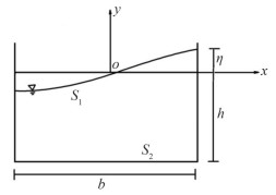Figure  1  Schematic sketch of the sloshing phenomenon in a rectangular storage tank

Download: Full-Size Img

If we assume inviscid, irrotational and incompressible fluid flow Euler equations apply (Ketabdari and Saghi, 2013a). Instead of modelling the problem for a moving storage tank subject to an acceleration vector of (a_x.a_y), an opposite acceleration is exerted to the fluid. For this case, the governing equations become:

The 2D incompressible continuity equation is also defined as:

Using velocity potential in Eq.3, the Laplace equation is becoming:

The conditions of incompressibility for the side/bottom boundaries and the free surface are defined as:

The Laplace equation and the dynamic free surface boundary condition are solved simultaneously using coupled boundary element-finite element methods. The results of the model are free surface displacement and potential function used for the estimation of pressure distribution and horizontal force exerted on the tank perimeter. To model the sloshing phenomenon, free surface boundary conditions and impermeable condition for side and bottom boundaries are considered as (Ketabdari and Saghi, 2013b):

To solve Laplace equation (Eq. 4) using BEM, the Green's theorem was applied resulting in

In this equation, c(x) is calculated as:

In this step, Green theorem is also used to replace domain integrals in Eq.(11) to boundary integrals as follows

By using the Linear shape functions (Ketabdari and Saghi, 2013b) we have

where

More detail about the parameters is presented in Ref. Ketabdari and Saghi (2013b).

To discrete and solve the dynamic free surface boundary condition (Eq. 7), finite element method was used. To do this, error correction term (D) is used to solve this equation as follows

To solve this equation by using Galerkin method and after discretisation of the equation, residual of equation 18 is estimated as

Total residual of j node in two adjacent elements should be zero. So:

By solving equations 14 and 25, free surface oscillation and pressure distribution on the tank perimeter are estimated.

3   Developed models

This section presents more details about ANN and GA.

3.1   ANN modelling

ANN are computational networks that simulate the nerve cells of the biological nervous system (Graupe, 2007). The perceptron is the basic building block of all ANN and possesses the fundamental structure of several weighted input connections. Those link to the outputs of several neurons. If we denote the summation output of the Perceptron as z_i and its inputs as x_ni, the Perceptron's summation relation is defined as:

The activation operation is defined by the so-called activation function f (z_i); where f is a nonlinear function yielding the i^th cell's output. In this paper the activation functions considered were respectively of sigmoid (S), hyperbolic tangent (T), and pure line (P) format as follows:

In this paper, different activation functions (AF) (Equations 22 to 24) were used for the hidden and output layers to generate the geometries of ANNs (see AF at Table 2). For instance, SP means that the sigmoid and pure line activation functions used in the geometry of ANN for the hidden and output layers, respectively. If the sway motion amplitude (a), angular frequency (ω), tank width (b), and water depth (h) are the input variables of the ANN model, the parameters η_max and F_x-max are outputs (Figure 2).

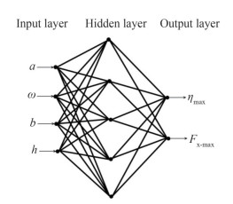Figure  2  Architecture of ANN used in this research

Download: Full-Size Img

Regarding the training of the ANN, the feed-forward back propagation (FFBPN) and multi-layer perceptron schemes have been applied. The flow chart of FFBPN is presented in Figure 3. The procedure was started with collecting the data and identification of parameters. The collected data was normalized within the range of 0 to 1. At the next step, by using 70 percent of data and Feed-Forward Back Propagation (FFBPN) method the network was trained. The train consist of two steps, forward step for input weights and the backward step for updating weights and errors. Then, network validated and tested by using 15 percent of data for each one.

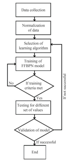Figure  3  Flowchart of FFBPN procedure

Download: Full-Size Img

3.2   GA modelling

The genetic algorithm is a method for solving optimization problems based on natural selection and the process that drives biological evolution. This algorithm repeatedly modifies a population of individual solutions so that individual populations was selected from the current population to be parents and uses them to produce the children for the next generation. The population evolves toward an optimal solution over successive generations. The genetic algorithm can be applied to solve a variety of optimization problems including in which the objective function is discontinuous, stochastic, or highly nonlinear that are not well suited for standard optimization algorithm. The genetic algorithm can address problems of mixed integer programming, where some components are restricted to be integer-valued. In the GA method at first the mechanism of turning every answer into a chromosome should be defined (Forrest, 1993). Then, a series of chromosomes that are answers to the problem are adopted as initial population. These sets are arbitrary and created by user randomness. Consequently, a genetic operation can be used to generate new genes known as the child. These operations can be categorized into two main types of crossovers and mutation. The concept of crossover rate and mutation rate can be used to select chromosomes who play the role of parents. The new population is created using the change of two genes, chromosomes, and the tree coding. A flow chart of GA is presented in Figure 4. The last generation of chromosomes for η_max and F_x-max are shown in Figure 5. In this figure, the generalized parameters d₀, d₁, d₂, and d₃ are represented by the variables a, ω, b, and h, respectively.

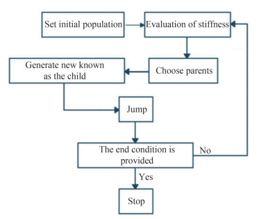Figure  4  Flow chart of GA

Download: Full-Size Img

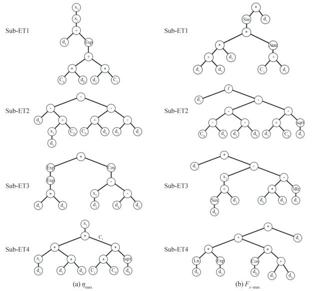Figure  5  The last generation of chromosomes

Download: Full-Size Img

4   Numerical model validation

The analysis simulated sloshing loads applied on a rectangular tank of width of 0.9 m and water depth 0.6 m exposed to a horizontal periodic sway motion of 0.002 m amplitude and 5.5 rad/sec angular frequency. At first instance, nodal displacement on the free surface and in contact with right hand sidewalls was evaluated for different mesh sizes. Mesh independency is evident for l ≤ 0.05 m. The nodal displacement results presented in time steps ∆t between 0.002 to 0.004 s and time step independency is evident for ∆t ≤ 0.002 5. Excellent comparison against the results of Nakayama and Washizu (1984) confirmed the validity of the solution (see Figure 6). The result of long-time histories is also shown in Figure 7, so that the maximum free surface oscillation is shown.

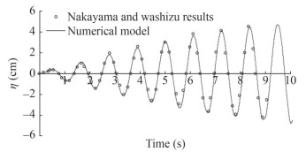Figure  6  Comparison between the NM and Nakayama and Washizu results (1984).

Download: Full-Size Img

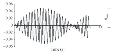Figure  7  Explanation of max free surface displacement.

Download: Full-Size Img

Figure 8 also demonstrates free surface profiles of sloshing induced flow in a rectangular tank in different time instants.

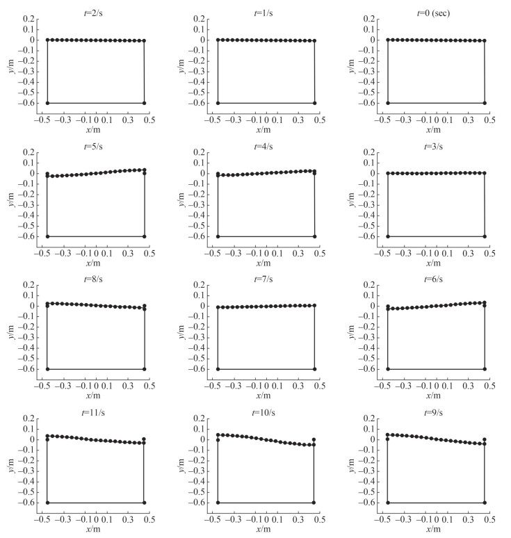Figure  8  Free surface profile for sloshing in a rectangular tank exposed to a horizontal sway motion in different times

Download: Full-Size Img

5   Results and discussion

In this paper, the rectangular storage tank of width (b) and water depth (h) was exposed to horizontal periodic sway motions as a_x = asin (ωt), and η_max and F_x-max were estimated by using the numerical model. Key results from determinist sloshing analysis are summarized in Table 1.Trained ANN were used to idealize sloshing pressures in a rectangular tank with b = 0.7 m and h = 0.9 m exposed a sway motion of 9 rad/s angular frequency. Table 2 summarizes results for a Number of Hidden Layer Cells (NHLC) corresponding to Activation Functions (AF) used in the hidden and output layers of the ANN. The error criteria were estimated as:

In the above equations η_{i, max-NM}, η_{i, max-ANN}, F_{i, max-NM}, and F_{i, max-ANN} were used to estimate η_max and F_x-max and n is the number of the cases simulated by ANN (see Table 2, n = 40).

Along the lines of the results presented in Figure 9, an ANN with sigmoid AF in the hidden and output layers and 7 neurons in the hidden layer present the optimum numerical fit.

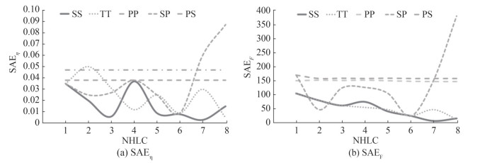Figure  9  Comparison of different terms for different ANNs

Download: Full-Size Img

In the GA based approach, the following equations for η_max and F_max were tested and resulted in:

The obtained formulas were used to estimate η_max and F_x-max for some test cases, and the results are summarized in Tables 3 and 4.

Predictions from ANN and GA for various cases are summarized in Tables 5 and 6, where $E_\eta=100 \frac{\left(\eta_{\max -\mathrm{NM}}-\eta_{\max -\mathrm{est}}\right)}{\eta_{\max -\mathrm{NM}}} ;$ $E_F=100 \frac{\left(F_{\max -\mathrm{NM}}-F_{\max -\mathrm{est}}\right)}{\left.F_{\max -\mathrm{NM}}\right)} ;$ the parameters η_max-est and F_max−est represent the max free surface displacement and horizontal force exerted on the tank perimeter. Based on these results, the maximum errors of ANN and GA were found to be in the range of 0.45%-14% with the error values of ANN lower (0.6%–6.8%) in most cases. It was therefore concluded that both ANN & GA represent with suitable accuracy both η_max and F_max predictions and therefore they could be implemented in methods and engineering tools used for the rapid assessment of sloshing loads in rectangular storage tanks.

6   Conclusions

In this paper, ANN and GA methods were used to predict η_max and F_x-max from liquid sloshing phenomenon in a rectangular storage tank. Statistical metamodeling was based on a potential flow FSI model that simulated the influence of periodic sway induced motion dynamics on a partially filled rectangular tank. Results showed that an ANN with sigmoid activation function in the hidden and output layers and 7 neurons in the hidden layer give the minimum errors. The maximum errors of GA were found to be in the range of 3.23%‒14.01% for η_max and 2.5%‒6.48% for F_max. The error values of ANN were lower, i.e., in the range of 0.45-6.88% for η_max and 0.66% ‒ 6.5% F_max. It was concluded that the proposed models represent with suitable accuracy both η_max and F_max predictions and therefore it could be implemented in methods and engineering tools used for the rapid assessment of sloshing loads in rectangular storage tanks.