1   Introduction

The recent advances in Computational Fluid Dynamics (CFD) for incompressible flow are gradually proving to be invaluable asset for design and analysis of ship, submarines, underwater missiles, low speed transport aircrafts and a wide variety of equipment design in process industry. Accurate prediction of turbulent flow is of great practical interest in the overall performance of ship hull to be designed. The understanding of the physics of fluid turbulence is far from complete and Reynolds Averaged Navier Stokes (RANS) methodology coupled to statistical turbulence model is often very useful and reliable for computation of statistically stationary turbulent flows.

Potential flow code which ignores the fluid viscosity, have been performed to simulate the fluid flow around an abitrary body like the ship hull. Mei et al. (2020) and Tu and Chien (2018b) computed the wave resistance by solving the non-linear free surface potential flow problem using a surface panel method. In case of advanced CFD code, the RANS equation is solved to simulate the free surface flow efficiently and to predict the different hydrodynamic behaviors including the total resistance of the ship hull (Ahmed, 2011). These numerical techniques also give an intense understanding of complex fluid flow under the realistic sea condition with lesser resource and time which assure an advanced area of design and optimization in ship industry (Korkmaz et al. 2015).

Campbell et al. (2022) used CFD method to study the change in ship's resistance as its trim and draft increases while moves through a restricted waterway. Hydrodynamic resistance increases by 10%‒15% with the increasing draft. The study also showed that the increased resistance can be compensated by varying the trim angle at low speeds. RANS simulation was performed varying Froude numbers and drafts to predict the resistance in calm water condition of container ship Islam and Soares (2019). This study revealed that forward speed and draft conditions strongly affrect the optimum trim condition for minumum resistance of container ship. Zha et al. (2014) numerically studied the wave making resistance of six different hull forms at two different speeds (12 kn and 16 kn) using naoe-FOAM-SJTU solver. All six hulls carry the same dimension, while the main distiguishing feature includes the local diffrence in bow and sterns. The numerical results showed that hull 3 which has a cruiser stern, experienced the less calm water resistance comparing the remaining hulls.

In the assesment of ship hydrodynamics where ship hulls advances in water waves, it is required to reslove the interface between water and air, a multi-phase problem and the fluid-structure interaction between fluids and hull also need to be taken into consideraion Frisk and Tegehall (2015). Likewise, the mutiphase flow problem is also crucial in the two-phase bubble flow, bubble interaction, bubble dynamics, etc., Sato et al. (1981), Zhang et al. (2023). However, in the fluid-flow problem around the ship hulls, there are two frequently used methods: interface tracking method, Li and Matusiak (2001) and interface capturing method, Hirt and Nichols (1981) are implemented to compute the free surface. Maronnier et al. (2003) presented the simulation of complex fluid flows with free surface solving for the unknowns: velocity and pressure. The mathematical problem was formulated following volume of fluid (VOF) method and a splitting algorithm was augmented to decouple the advection and diffusion. A good agreement was found with this numerical approcah when compared with experiment. Cao and Wan (2015) studied wave run-up on a circular cylinder using an incompressible two-phase flow solver naoe-FOAM-SJTU. VOF method was added to capture the air-water interface. Numerically simulated wave force and wave run-up were compared with experimental data, moreover, the free surface evolution, pressure contour, vortex shedding were also presented.

Azcueta (2000) computed turbulent free-surface flows around ships using Reynolds Averaged-Navier Stokes equations solver ICCM-Comet. An interface capturing scheme was used to determine the shape of the free surface. Two test cases: Wigley and Series 60 hulls were investigated at Froude no. 0.267. Obtained results showed a good agreement with the experimental results. Zhao et al. (2005) numerically investigated viscous flow around the ship with free surface solving the Reynolds-Averaged Navier-Stokes (RANS) equations with an acceptable level of accuracy. Perez et al. (2008) studied resistance and wave profile at six Froude numbers with the application of CFD code ANSYS-CFX 11.0. The study showed a good agreement for resistance, but the wave profile along the hull did not improve.

Pranzitelli et al. (2011) simulated free surface flow around a semi-displacing motor yacht advancing steadily in calm water. The volume of fluid method (VOF) was implemented in Reynolds-Averaged Navier-Stokes (RANS) equations and this VOF method correctly predicted both the free surface shape and the total resistance. Ebrahimi (2012) carried out a numerical study on a model of bulk carrier and calculated the total resistance using ANSYS FLUENT 13 based on finite volume method (FVM). Applying volume of fluid method RANS equations are solved and a fully structured mesh generated in GAMBIT pre-processing software was used. Yao and Dong (2012) computed sinkage and trim by equating the vertical force and pitching moment to the hydrostatic restoring force and moment. Sarker et al. (2017) predicted calm water resistance, sinkage and trim of a modern surface combatant using finite volume method (FVM) code. The study used ONR (Office of Naval Research) Tublehome model 5 613 fully appended with skeg, bilge keels and rudder, to conduct the CFD simulation and presented the uncertainty analysis as well.

Atreyapurapu et al. (2014) computed the wave pattern and the total resistance (shear and pressure resistances) for a container ship using STAR-CCM+ software and modelling the flow with Realizable k − ε and shear stress Transport (SST) k − ε turbulent models. The effects of sinkage and trim were also studied and the method was found to be stable and was believed to predict the resistance for any ship with or without trim and sinkage. Ozdemir et al. (2014) carried out an experimental and computational research for a fast ship model. The Reynolds Averaged Navier Stokes (RANS) equations and the nonlinear free surface boundary conditions were discretized by means of an overset grid finite volume scheme. The experiments were performed at Istanbul Technical University Towing Tank basin. In the numerical turbulent flow calculations, the relationship between the Boussinesq's hypothesis of turbulence viscosity and the velocities were obtained through the standard k − ε turbulence model. Simulations of turbulent free surface flows around the model were performed using Star CCM+ solver where Volume of Fluid (VOF) model were used to capture the free surface between air and water. The total resistance of the ship model was compared with the experimental results. Bow and aft wave form developments were investigated qualitatively. For Froude numbers less than 0.25, the computations were found to be well satisfactory, giving efficient and accurate tool to predict curves of resistance. For relatively higher speeds greater than 0.25, a low Reynolds number turbulence model could be more suitable to predict the resistance.

Tu et al. (2018c) predicted ship resistance, sinkage and trim in calm water using unsteady RANS method in which performing some simulations on a sequence of systematically refined grid, the effects of grids on simulation results were investigated. Bahatmaka and Kim (2018) presented a numerical investigation of ship resistance of Indonesian traditional fishing vessel. The OpenFOAM was used to solve the unsteady incompressible RANS equations for the ship resistance. The volume of fluid (VOF) method is used to capture the free surface. The results of KCS model were compared to the experimental results and showed very good agreement. Tarafder and Mursaline (2019) simulated the turbulent flow around two-dimensional bodies using the finite volume method with non-orthogonal body fitted grid. The k − ε turbulence model and wall functions were used to bridge the solution variables at the near wall cells and the corresponding quantities on the wall. The solution was carried out using the SIMPLE algorithm with a simplified pressure correction equation for collocated arrangement for scalar and vector variables.

Ship Hydrodynamic performances such as total drag, sinkage and trim were evaluated using CFD simulation of a planning hull Pacuraru et al. (2022). A proper grid size and time step followed by convergence test was selected to perform the further assesment on hydrodynamic flow parameters under several geometric configurations such as tunnels, spray rails and whiskers. Feng et al. (2021) studied parametric hull form optimization aiming for miminum resistance in calm water and in waves. The optimized hulls were subjected to the regular head waves and obatined added wave resistance were compared with experimental results. Non-linear potential flow boundary element method was employed to compute the flow around the hulls. The results showed that wave resistance at lower speeds decreased by a larger amount than at medium and higher speeds. Ship-to-ship hydrodynamic interaction was performed using CFD code with the comparison results against experimental data and panel method as well Wnęk et al. (2018). The free surface was modeled both as a rigid wall and a deformable surface while working with the both inviscid and viscous flows. The inviscid rigid wall model underprediced the surge interaction force and that was improved considering the viscosity in the flow model. Viscosity consideration in the free-surface flow model enhanced the improvements, however, demanded the slower calculations.

Kwag (2001) characterized the flow fields around a high speed catamaran for Froude numbers ranging from 0.2 to 1.0. A rectangular grid system based on the Marker & Cell method was applied for performing the computation. The H-H grid topology was used to treat the free surface movement. A pentamaran model of Wigley hull form was investigated experimentally by Yanuar et al. (2019) to characterise the resistance and interference comparison between the symmetric and asymmetric hull configurations. The total resistance coefficients was found in steady trend in the symmetric case while compared with the asymmetric case. Zhao et al. (2023) performed numerical analysis using finite volume method on the monohull and pentamaran in viscous flow domain. Calm water and regular wave conditions were analyzed employing the dynamic fluid-body interaction (DFBI) and overset mesh respectively. Research stated that calm water resistance contribution from the side hulls of the pentamaran can be neglected in the high speed ranges. In the analysis of regular wave, monohull experienced a non-linear total resistance compared to the pentamaran hull which experienced linear behavior under same wave condition.

The main objective of the present study is to numerically investigate the fluid flow around KCS, Series 60 and Catamaran hulls. Finite volume method (FVM) based commercial CFD software STAR-CCM+ is used to perform the simulation. This commercial code uses the SIMPLE algorithm to solve the discretized governing equations. A well-known k − ε two equations turbulence model is used to give the closure of Reynolds Averaged Navier Stokes (RANS) equation to extract the velocity and pressure field numerically. The volume of fluid (VOF) multiphase model is implemented to determine the position of free surface between air and water phases. In this model velocity, pressure, and temperature are shared by all phases. Wall function is employed to the wall boundary to the hull surface to resolve the near wall flow.

The obtained numerical results that include total resistance, sinkage, trim, wave profile and wave pattern are compared with the available results (Kim et al., 2001; Zou and Larsson, 2014; Takeshi and Hino, 1987). A good consistency level is found between the computational and experimental results. The three different mesh arrangements are also generated to determine the dependence of results on the quality of grid.

The paper is organized as follows: section 2 provides an overview of mathematical modeling of fluid flow around the ship hull with the boundary conditions specifications. Section 3 focuses on discretization of govering equations by means of FVM method. In section 4, numerical results include total resistance, sinkage, trim, wave profile and wave pattern of KCS hull, Series 60 hull, and catamaran hull are presented with grid convergence and verification studies.

2   Mathematical modeling of ship flow

2.1   Governing equations of RANS

The governing equations of 3-dimensinonal turbulent flows for an incompressible fluid around a ship can be represented by the continuity and momentum equations as follows:

where ρ and μ are the density and the kinematic viscosity of the fluid. p is the pressure exerted by the fluid and u, v, w are the instantaneous velocity components along the x, y and z directions respectively. Turbulence consists of random fluctuation of various flow properties and following Reynolds (1895) all the flow properties are replaced by the sum of mean and fluctuating parts. Taking the time average of Equations 1 ‒ 4 the Reynolds-Averaged Navier-Stokes (RANS) equations can be expressed as

In Equations 6‒8 there are six apparent unknown stresses and the stress tensor of these Reynolds stresses is defined by (STAR-CCM+ user guide, 2011):

The eddy viscosity model (Andreasson and Svensson, 1992) uses the concept of a turbulent viscosity μ_t to model the Reynolds stress tensor as a function of mean flow quantities. The most common model proposed by Boussinesq (1877) can be written as:

where S is the strain tensor and is defined by

The turbulent kinetic energy is defined by $k=\frac{1}{2}\left(\overline{u^{\prime} u^{\prime}}+\right.$ $\left.\overline{v^{\prime} v^{\prime}}+\overline{w^{\prime} w^{\prime}}\right)$. The $k-\varepsilon$ turbulence model is a two-equation model that solves transport equations for the turbulent kinetic energy $k$ and its dissipation rate $\varepsilon$. The standard equations for $k$ and $\varepsilon$ are:

where, $\sigma_{k}$ (Turbulent Prandtl number) is a closure coefficient, $\mathrm{v}_{\mathrm{t}}\left(=C_{\mu} k^{2} / \varepsilon\right)$ is the kinematic eddy and $\mathrm{Q}$ is the rate of production of $k$ due to Reynolds stress defined as:

The standard values of constants used in k − ε turbulence model are:

The use of standard k − ε two equations turbulence model is reasonably robust and reliable near solid boundaries and recirculation regions like ship boundary layers. The pressure and velocity components are come out from Eqs. 5‒8 using well-known SIMPLE algorithm and then the kinetic energy k and the energy dissipation ε are obtained from Eqs. 12‒13.

2.2   Volume of fluid (VOF) method

The free surface flow generated at the interface of multiphase, e.g., air and water, can be modeled commonly used volume of fluid (VOF) method. In the VOF method, velocity, pressure, and temperature fields are shared by all immiscible phases present in a control volume, STAR-CCM+ user guide, 2011. In addition to the conservation equations, the filled fraction of each control volume is governed by the VOF transport equation as follows (Wu et al., 2011):

where, α is the volume fraction defined as:

For each control volume, the summation of volume fraction of each phase should be one. For example, in this case, the summation of volume fraction of air (α_a) and water (α_w) is:

With the volume fraction definition, a single momentum conservation equation for multi-phase flows is solved, where field properties are being shared by phases. The momentum equation is dependent on the equivalent fluid properties, which are extracted from the constituent phases and volume fraction. The density (ρ) and viscosity (μ) in the control volume can be estimated as following:

where ρ_w, μ_w and ρ_a, μ_a are the water density, viscosity and air density, viscosity, respectively.

2.3   Boundary conditions

The general view of the computational domain including the ship hull and the notations of its boundary conditions is depicted in Figure 1. The computational domain is split into two sub-domains (air and water) and has an interface between the flow fluids. This entire computational domain is bounded by six boundary surfaces such as inlet, outlet, side, symmetry, top and bottom. The boundary conditions imposed on each surface are described below (Masuko and Ogiwara, 1990):

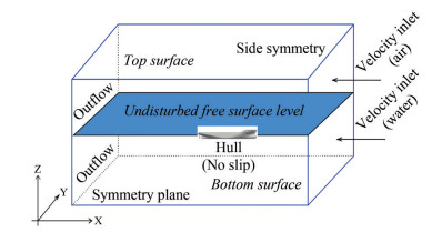Figure  1  Computational domain and its boundary conditions

Download: Full-Size Img

(a) Inlet boundary: Like the inviscid flow problem, the initial velocity components in x, y and z direction are selected as,

(b) Outlet boundary: The pressure at outlet is assumed to be the hydrostatic on the free surface and the shear forces are prescribed zero to meet the criteria of stress continuity equation.

(c) Side and Symmetry boundary: The axis of symmetry of the computational domain and the surface of symmetry (side) plane can be considered as the boundaries. The net flow across the symmetry is zero and hence the velocity including the turbulent quantities normal to the boundary is set to zero.

(d) Top and Bottom boundary: The top and bottom boundaries are considered as the wall type and can be written as,

(e) Ship hull: The velocity components (no-slip) and the turbulent quantities on the hull are set to zero.

(f) Wall function: The wall function emulates the behaviour of the flow inside the boundary layer. On the first grid point of the body k and ε become:

Towards the outer part of the viscous sub layer and the buffer layer, the turbulence is rapidly increased by the production of turbulent kinetic energy. With the use of standard k − ε turbulence model, additional wall functions are necessary to bridge the solution variables in the viscosity affected region. The velocity in the log-law region varies logarithmically with y + as given by Eq. 22. Although there is a slight variation in the values of universal constants in the literature, according to Stanford conventions suggest the von Karman constant κ as 0.41 and the equation constant B as 5.0.

where u⁺ is the stream wise velocity is non-dimensionalized by the friction velocity u_τ. y⁺ is the normalized wall distance such that y⁺ = yu_τ/ν. At the upstream boundary, the uniform flow condition is used. At the downstream boundary, zero derivative condition in x-direction is used and the pressure is taken as hydrostatic. At the symmetry plane boundaries zero derivative condition in the normal directions are utilized.

2.4   Resistance

The ship experiences the forces both from the air and water. The skin frictional resistance component comes from the shear forces acting tangentially on the hull surface. The pressure normal to the hull is responsible for pushing the water from its surface and is the source of residuary resistance component. The traditional RANSE solver software divides the total resistance into two parts that can be formulated as

where C_T denotes total resistance coefficient while C_R is the residual resistance coefficient and C_F is frictional resistance coefficient. The resistance coefficients can be nondimensionalized as:

where x in the subscript of C_x may refer to any resistance component. The residuary resistance coefficient can be further split into

where C_W and C_VP are the wave and viscous pressure resistance coefficients respectively. Note that a fully submerged body in a fluid domain of infinite depth has zero wave resistance (no free-surface effect) and the pressure resistance coefficient in this case becomes equal to the viscous pressure resistance coefficient.

2.5   Sinkage and trim

To get the resultant force and moment for sinkage and trim, STAR-CCM+ simulates the 2-DOF (degree of freedom) motion of the rigid body after solving the governing equation and finds the new position of the body. Dynamic Fluid-Body Interaction (DFBI) module allows calculating the free motion in which selected motions are taken as active to be calculated and other motions are remain as constrained. The input value for the moment of inertia and the center of mass are supplied at the initial stage of simulation. The translational motion of the center of mass is governed by:

where m represents the mass of the body, f is the resultant force acting on the body and V is the velocity vector of the center of mass. The rotational motion of the body is governed by:

where M is the tensor of the moments of inertia, ω is the angular velocity of the rigid body and n is the resultant moment acting on the body. The tensor of the moments of inertia is expanded as:

Only the principal diagonal components (M_xx, M_yy, M_zz) have the non-zero values in the simulation. The governing equations for rotating and translating body are given, which are solved by DFBI translation and motion solver to calculate the sinkage and trim of the hull.

3   Numerical modeling by finite volume method

The RANS equations are highly complex and cannot be solved analytically except in the special case. However, the commercial code STAR-CCM+ is based on finite volume method where the differential equations are converted into a system of linear algebraic equations and then applied at some discrete locations in space and time.

Introducing a transport variable ϕ the three-dimensional form of RANS equations for the conservation of mass, momentum, turbulent kinetic energy k and its dissipation ε can be converted into a general form of transport equation as

For continuity:

For momentum:

For turbulence:

Γ is the diffusion coefficient and S_ϕ is the source term. The approximation of the time derivative term $\partial \phi / \partial t$ is done by applying the first-order forward-difference (Tu et al. 2018a) scheme.

Δt is the incremental time step and the superscripts n and n + 1 denote the previous and current time levels respectively. Applying finite volume method, the discretized form of the generic transport Eq. 33 can be written as

This is a fully implicit scheme and the property ϕ at the center of the cell can be obtained applying SIMPLE algorithm.

4   Results and discussion

In the present study the three-dimensional flow around three types of ship hull forms such as KCS, Series 60 and a catamaran is simulated using RANS based code STAR-CCM+. The VOF model simulation is used to capture the free surface between air and water. The standard k − ε turbulence model with near-wall function is used to describe the velocity profile near the wall. For each type of hull appropriate fluid domain is specified following ITTC (2011) criteria. The numerical results include total resistance, sinkage, trim, wave profile and wave pattern will be presented and discussed in this section.

4.1   KRISO container ship (KCS)

KRISO container ship (KCS) is usually chosen as a benchmark for flow computations. The origin of the coordinate system is located at an undisturbed free surface at midship so that the undisturbed incident flow appears to be a streaming flow in the negative x-direction. The z-axis is vertically upward, and the y-axis extends to portside. The size of one-half of the computational domain is − 2.97 L < x < 1.97 L, 0 < y < 2.47 L, − 1.0 L < z < 0.17 L and is considered due to vertical plane symmetry that leads to reduce the number of element and to require less time to converge the problem. Due to the complexity of geometry of the ship at bow and stern, generating good, structured grids is not only very difficult but also very important in getting reliable numerical solutions. The KCS hull is firstly analyzed at the fixed condition to get the calm water resistance and then allowed to move freely to calculate sinkage and trim. The principal particulars of the KCS model are given in the Table 1 and its discretized view is given in Figure 2.

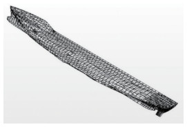Figure  2  Surface mesh applied on the KCS hull

Download: Full-Size Img

A trimmed cell mesher technique is used to produce hexahedral cell and prism layer mesher model is applied to resolve accurately the turbulent flow near the solid wall of the hulls as shown in Figure 3. Near the bow and stern, block structured volumetric cells are created to get better mesh quality. To capture the free surface efficiently a thin rectangular block is created with high mesh resolution which plays an important role to generate the wave pattern on the free surface as shown in Figure 4.

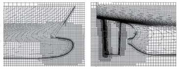Figure  3  Mesh applied at the bow and stern region of KCS hull

Download: Full-Size Img

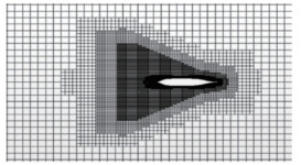Figure  4  Refined mesh at the free surface

Download: Full-Size Img

Special care is also taken away from the stern of the hull to capture the free surface wave more accurately.

Determination of the velocity gradients normal to the wall boundary has a remarkable effect on the accurate prediction of the flow features. Prism layer allows resolving these velocity gradients and its thickness is a region that governs a lot of key characteristics to predict the different hydrodynamic behaviors. The first prism layer height normal to the solid wall is determined by y⁺=60 and using a stretch factor 1.3 the size of the progressive layers are calculated as shown in Figure 5. The size of the last layer of the prism should be the closet size to the core mesh. The numerical values of layer thickness and the overall thickness are shown in Table 2.

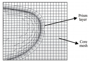Figure  5  Generated prism layers with the core mesh

Download: Full-Size Img

The discretized view of the computational domain is shown in Figure 6. Three different mesh arrangements categorized as fine, medium, and coarse mesh corresponding to cell numbers 1 057 126, 531 014 and 303 224, respectively, are applied on this computational domain.

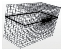Figure  6  Computational domain (36 m×18 m×27 m) of the KCS hull

Download: Full-Size Img

The flow velocity is given equal to 2.197 m/s corresponding to Froude number 0.26. In accordance with the guideline of ITTC (2011), the value of time step Δt is taken from the following mathematical relationship:

where L is the length between perpendicular and U is the flow velocity along the x-direction. Using a time step of 0.03 the convergence time history of resistance is drawn in Figure 7. It is observed that at the very beginning of time, the fluctuation rate is very high. But after elapsing certain period, fluctuating becomes very low and then solution is being converged. Among them frictional resistance converges very fast.

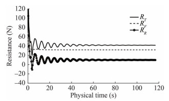Figure  7  Convergence history of frictional, residual, and total resistance

Download: Full-Size Img

Figure 8 shows a comparison of the total resistance co-efficient with the experimental results of Kim et al. (2001). At a very low Froude number the deviation between CFD and EFD (Kim et al., 2001) results is high but the discrepancy between these two is low at relative higher Froude number. The overall pattern of the resistance coefficient is quite satisfactory with the experimental results. The relative error between CFD and EFD values are given in Table 3.

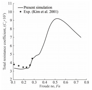Figure  8  Comparison of total resistance coefficients of KCS hull

Download: Full-Size Img

The present simulated wave pattern for Froude no. 0.26 is compared with that of Experiment Fluid Dynamics (EFD) as shown in Figure 9. A good agreement in terms of wave height and its position is found which assures the accuracy of CFD analysis around the hull form.

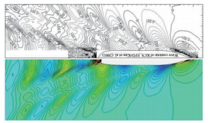Figure  9  Comparison of wave pattern of KCS hull between CFD (lower part) and EFD (upper part)

Download: Full-Size Img

The wave profile of the KCS hull is compared with the experimental data of Kim et al. (2001) and is shown in Figure 10. There is a very little discrepancy found at the bow and stern of the hull and these are probably mainly due to the poor meshing refinement. Since stern and bow sides are more complicated shape than any other region, a very strong mesh refinement would give better results. Wave height and location along the hull both are normalized by the length of the hull.

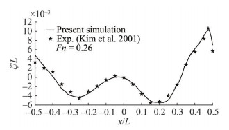Figure  10  Wave profile along the KCS hull at Fn=0.26

Download: Full-Size Img

Transverse wave cut is taken at 1.098 m from the center line of the ship and is presented in Figure 11 with the experimental data. A good agreement is found between the two-wave cut results.

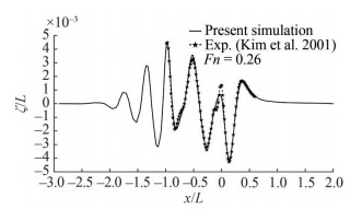Figure  11  Transverse wave cut at y=1.098 m from center line

Download: Full-Size Img

To investigate the dynamic behavior (in this case sinkage and trim), the KCS hull is simulated at free condition. Hull model is allowed to translate in the vertical direction and to rotate about the transverse axis. In the DFBI modeling, the release and the ramp time are chosen 1.0 sec and 5.0 sec. Release time gives sometimes to the fluid flow to be initialized before the motion calculation begins. Force and moments are applied on the hull body at the Ramp time and at this time solutions are carried out by reducing the oscillation. The simulation results for sinkage and trim are shown in Figure 12(a~b). A good agreement is found with the experimental results (Zou and Larsson 2014). Relative error analysis is also given in Table 4.

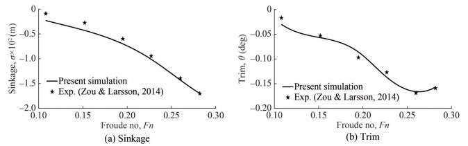Figure  12  Comparison of Sinkage and Trim for KCS hull

Download: Full-Size Img

Applying the grid refinement ratio $r=\sqrt{2}$ (value recommended by ITTC quality manual) grid dependency study is conducted using three different grids such as coarse (grid no. 3), medium (grid no. 2) and fine (grid no. 1) corresponding to the cell numbers 303 224, 531 014 and 1 057 126 respectively. The methodology discussed by Stern et al. (2001) is applied here for the study. The hull is run at same speed and all other set up kept as same except the mesh density. The grid properties with the corresponding numerical results are given in Table 5.

The simulated results of KCS hull for three numbers of grids are given in Table 6 with respect to the relative solution changes (ε), relative error (E%D) and EFD (D). The convergence ratio R_G, order of accuracy p_G, correction factor C_G and the numerical uncertainty U_SN are also given in Table 7.

Figure 13 shows a grid dependency study of wave profile along the hull for three number of mesh arrangement namely the grid 1 (Finest), grid 2 (Medium), and grid 3 (Coarse) respectively and a satisfactory agreement is found with the experiment results of Kim et al. (2001).

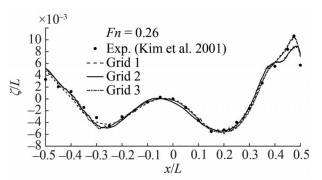Figure  13  Grid dependency study of wave profile of KCS hull

Download: Full-Size Img

4.2   Series 60 (C_B = 0.6)

The principal particulars of Series hull are given in Table 8 and its surface mesh is shown in Figure 14. The size of one-half of the computational domain is − 2.6 L < x < 1.5 L, 0 < y < 2.0 L, − 1.5 L < z < 0.2 L and is considered due to vertical plane symmetry as shown in Figure 15.

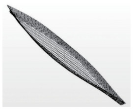Figure  14  Surface mesh of the Series 60 hull

Download: Full-Size Img

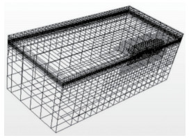Figure  15  Computational domain of Series 60 hull

Download: Full-Size Img

The total resistance coefficients for various Froude numbers ranging from Fn=0.20 to 0.72 are computed and then compared with the experimental results (Takeshi and Hino, 1987) as well as Karim and Naz (2017) as shown in Figure 16. A good agreement is found among the results.

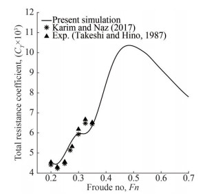Figure  16  Comparison of resistance of Series 60 hull

Download: Full-Size Img

Figure 17 dictates a change of wave contour for various Froude numbers and Figure 18 shows a comparison of computed wave profile with the experimental results (Gadd 1976).

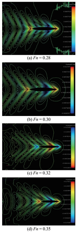Figure  17  Wave pattern for Series 60 hull at different Froude numbers

Download: Full-Size Img

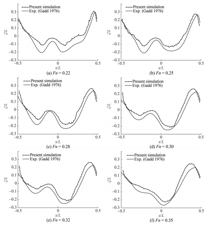Figure  18  Wave profile along the Series 60 hull at different Froude numbers

Download: Full-Size Img

4.3   Catamaran hull

The catamaran hull is composed of two identical Wigley mono hulls and has the hull separation to length ratio (s/L) is 0.4. Each mono hull is 3 m in length, 0.3 m in breadth and 0.187 5 m in draft. The size of one-half of the computational domain is − 3.5 L < x < 1.5 L, 0 < y < 1.67 L, − 1.0 L < z < 0.33 L and is discretized by 2 957 198 number of hexahedral cells as given in Figure 19.

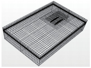Figure  19  Computational domain of the Wigley catamaran hull

Download: Full-Size Img

For the catamaran shown in Figure 20 special care is taken in case of separation of the hulls where the highly complex flow likely to be generated. This is done by creating another rectangular volumetric block with stronger mesh refinement and at the free surface mesh refinement is also taken as refined mesh.

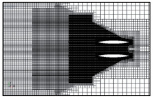Figure  20  Cluster mesh in the region of hull separation and in the wake

Download: Full-Size Img

The wave-making resistance of the catamaran hull is shown in Figure 21 and exhibits broadly similar trends to those of the published monohull results as well as the experiment of Insel and Molland (1992) and numerical results of Tarafder and Suzuki (2007).

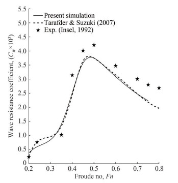Figure  21  Wave resistance coefficient comparison of Wigley catamaran hull (s/L=0.4)

Download: Full-Size Img

The wave contours at various Froude numbers such as 0.35, 0.40, 0.50 and 0.60 for a catamaran of s/L=0.4 are shown in Figure 22. From these figures it is observed that the effect of wave interference between the two mono-hulls is trivial due to large separation ratio s/L=0.4 and the pattern is likely to be similar as the mono hull. For a catamaran of smaller hull separation (s) to length (L) ratio, the transverse wave becomes dominant over the divergent wave (Kwag, 2001).

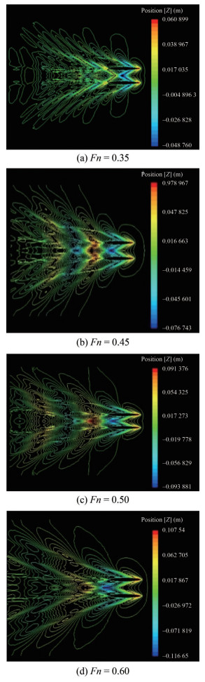Figure  22  Wave pattern at different Froude numbers of Wigley catamaran (s/L = 0.4)

Download: Full-Size Img

When this s/L ratio value becomes extremely smallest, the wave interference between hulls becomes so larger and the dominant transverse waves are circulated from the outer side of the hulls.

Figure 23 presents a comparison of wave profiles at outer and inner side of a catamaran hull of s/L=0.4 for four different Froude numbers 0.35, 0.45, 0.50 and 0.60, respectively.

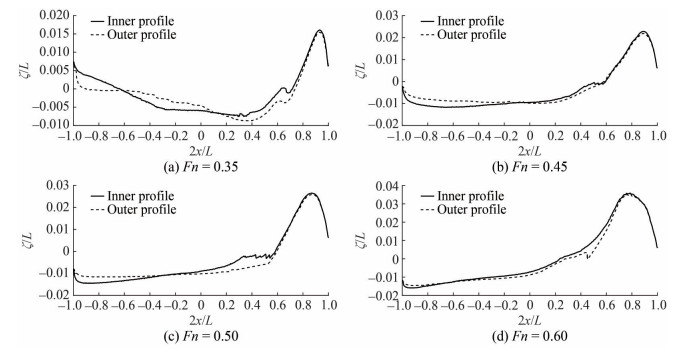Figure  23  Wave profile along the catamaran hull (s/L = 0.4)

Download: Full-Size Img

The difference in magnitude between the inner and outer wave profile of the catamaran is low due to higher s/L=0.4 that leads to trivial wave interference. At the bow side the wave height of inner profile is slightly greater than that of the outer wave profile for every Froude number. This is so because the effect of the wave interference even though in small scale.

5   Conclusions

In this present study, the fluid flows around KCS, Series 60 and a catamaran hull are investigated numerically using a commercial CFD code STAR-CCM+. The k-ε turbulence model in connection with SIMPLE algorithm is chosen to extract the velocity and pressure fields. The present study is done with the calm water conditions; hence, future study can be extended including both regular and irregular waves of real sea environment. The separation between catamaran hull plays significant role in wave interference effects. The further analysis with different hull separations can lead to optimize design of catamaran hull. The following conclusions can be drawn from the analysis:

a) The standard k-ε turbulence model can be adopted as powerful tool to analyze the ship flow (resistance, sinkage, and trim) except for the case where the flow separation occurs.

b) The diverging waves radiating from the bow and stern are well predicted and look very similar to the wave pattern in deep water (Kelvin wave pattern).

c) As expected, the finer are the grids, the better is the accuracy found with a cost of longer computation time. Reducing the grid size provides better mesh representation at the bow and aft of the ship model. However, it also increases the computation time drastically, and sometimes the CPU may not be able to compute the huge amount of data because of memory deficiency. Several grid refinement studies are performed, and the optimum grid size were chosen for resistance calculations.

d) The magnitude of the wave profile on the inner side of the catamaran hull is slightly higher than that of the outer side at the first crest of the bow. This difference is mainly due to the wave-interference effects.

e) In general, the agreement between calculation and experiment tends to become worse with the increasing Froude number. Future work can include more study cases and quantitative analysis to address this issue.

f) The predicted numerical results using STAR-CCM+ demonstrate the capability of efficient using commercial CFD code while comparing the results against experiment. Therefore, current analysis with CFD code analysis can be used to make necessary improvements and corrections in the early stage of design and furthermore, it can lead to optimize the hull form.

Nomenclature