1   Introduction

In recent decades, the mathematical study of the performance of breakwaters has received significant attention in order to protect coastal regions and attenuate wave energy. There has been a rise in interest in the use of flexible breakwaters as an alternative to the more conventional rigid type breakwaters in coastal regions, particularly where a poor sea bed exists. However, it is necessary for the transmitted and reflected wave heights to be small, which is why porous structures can be used effectively to dissipate wave energy. Moreover, flexible breakwaters are reusable and cost-effective for protecting marine structures from destructive waves. Additionally, these types of breakwaters generate fewer hydrodynamic forces. Therefore, the study of the performance of flexible porous breakwaters in predicting wave motion is of great importance in coastal engineering practice.

Meanwhile, fair developments have been made in both the theoretical and experimental investigation of the porous breakwater, with and without flexibility. Several mathematical tools have been formulated to deal with various shapes of porous barriers. A porous wave maker theory was developed by Chwang (1983) to study the small amplitudes of water waves raised by horizontal oscillations of a permeable barrier in uniform bottom. The hydrodynamic performance of submerged and surface-piercing permeable barriers in deep water was studied by Sahoo (1998) using logarithmic singular integral equations. Furthermore, Lee and Chwang (2000) used the least square method to analyze the effect of partial porous breakwaters of various configurations on the scattering of water waves. This analysis was extended by Sahoo et al. (2000), who studied the trapping and generation of normally incident water waves by considering an impermeable back wall. The trapping of water waves by two different kinds of porous flexible breakwaters, namely bottom standing and surface piercing, was studied by Yip et al. (2002). Williams and Wang (2003) investigated the hydrodynamics of flexible breakwaters to enhance the effectiveness of wetlands habitat restoration projects. Li et al. (2006) investigated the values of the porous effect parameter of thin porous breakwaters theoretically and experimentally. The problem of water wave scattering by a porous breakwater was converted to a second-kind hypersingular integral equation by Gayen and Mondal (2014) and analyzed for finite and infinite depth water. Using Babinet's principle, Manam and Sivanesan (2016) analyzed wave scattering by a porous barrier in deep water by demonstrating a connection between two wave potentials. Furthermore, a detailed study on oblique wave scattering and trapping was carried out by Koley et al. (2015) and Kaligatla et al. (2015) by converting the boundary value problem into a system of three Fredholm-type integral equations using Green's function. Das and Bora (2018) analyzed the performance of reflection and transmission coefficients for two vertical unequal porous breakwaters. Krishna et al. (2023) studied the interaction of oblique waves with porous block in the presence of thin permeable breakwater. Recently, Krishnendu and Balaji (2020) conducted a numerical and experimental investigation on wave trapping by a porous breakwater placed in front of an impermeable rigid wall. Gupta et al. (2022) analyzed the scattering of water waves by two vertical porous flexible plates using Havelock's theorems for water waves.

In the previously mentioned articles, hydrodynamics of water waves were analyzed in uniform water depth however significant changes in wave characteristics occur due to bottom variation. Hence, there is a need to understand the refraction diffraction effects caused by the varying bottom. The refraction diffraction effect induced by varying bottom is examined with the help of the mild-slope equation which was derived by Berkhoff (1973) by using vertical averaging technique. Next, Chamberlain and Porter (1995) derived a modified mild-slope equation by employing the variational principle. The study of water wave interaction with a breakwater in the presence of varying bottoms is often important to understand the characteristics of waves to address more realistic physical problems. Suh and Park (1995) studied the reflection and transmission coefficients by porous breakwater in the presence of step-type bottom. However, they did not ensure the conservation of mass at the bottom slope discontinuity. The mass conserving jump condition is deduced by Porter and Staziker (1995) by addressing the effect of evanescent mode in the study of Chamberlain and Porter (1995). The application of modified mild-slope equation along with jump condition can be seen in the article of Behra et al. (2015) who studied oblique wave trapping by porous breakwater in the presence of step-type bottom. Further, their model was extended by Kaligatla et al. (2018) who investigated the oblique wave scattering by multiple porous breakwaters in the water of varying depth. Recently, Venkateswarlu and Karmakar (2020) examined the significance of variable step-type bottom characteristics on wave trapping by stratified porous breakwaters.

The objective of the present article is to investigate the wave trapping and scattering by flexible porous breakwater by taking into account the effect of the varying bottom. The porous breakwater is assumed to be fixed at the bottom and placed in front of impermeable wall. The problem is examined under the framework of small amplitude water wave theory and Darcy's law is used to study flow past porous medium. The present physical problem is modeled by employing the MMSE of Chamberlain and Porter (1995) for the region of the varying bottom along with eigenfunction expansion method for flat bottom. The obtained solution in each region is matched at interface along with mass conserving jump condition at slope discontinuity. The system of algebraic equations is obtained and solved numerically to determine the unknown coefficients. Various physical quantities such as reflection coefficient, and wave force exerting on breakwater and wall are plotted and analyzed for several parameters. Moreover, several outcomes associated with the present problem are analyzed, validated, and compared with the known results available in the literature.

2   Statement of the boundary value problems

In the present work, the interaction between oblique waves and thin flexible breakwater is studied in the presence of varying bottom. Oblique wave trapping and scattering by thin porous flexible breakwater is formulated through Cartesian coordinate system (x, y, z). The present Boundary Value Problem is modeled in the framework of small amplitude water-wave theory. The free surface is assumed to be undisturbed and lying on the xy−plane and z−axis being in a positive upward direction. The bottom of sea is assumed to be impermeable and varying bottom at z = − h₂ (x) is spanned over 0 ≤ x ≤ L is connected by two uneven constant depth levels of z = − h₁ and z = − h₃ with h₃ < h₁. The flexible porous breakwater is fixed at z = − h₃ at x = L + L₁ with and without wall on the lee side. According to the geometry of problem, whole fluid region is divided into four sub-regions as shown in Figure 1. The first region is defined as Ω_I ={− ∞ < x < 0, − ∞ < y < ∞, − h₁ ≤ z ≤ 0}, second region is Ω_II ={0 ≤ x ≤ L, − ∞ < y < ∞, − h₂ (x) ≤ z ≤ 0}, third region is Ω_III ={L ≤ x ≤ L + L₁, − ∞ < y < ∞, − h₃ ≤ z ≤ 0} and the last region is Ω_IV ={L + L₁ ≤ x ≤ ∞, − ∞ < y < ∞, − h₃ ≤ z ≤ 0} for scattering problem and Ω_IV = {L + L₁ ≤ x ≤ L + L₁ + W, − ∞ < y < ∞, − h₃ ≤ z ≤ 0} for trapping problem. The fluid in each region is assumed to be inviscid, incompressible and the motion is irrotational and wave motion is assumed to be simple harmonic in time with angular frequency ω. With all these assumptions, fluid motion can be described in terms of velocity potential, Φ_r = $\operatorname{Re}\left\{\phi_r \mathrm{e}^{-\mathrm{i}\left(\mu_y y+\omega t\right)}\right\}$ for r = I, II, III, IV with i = $\sqrt{-1}$ and μ_y = β₀ sin θ, where β₀ being the wavenumber of incident wave.

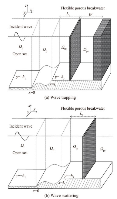Figure  1  Depiction of wave trapping and scattering by a flexible porous breakwater in water of undulating bottom

Download: Full-Size Img

The spatial velocity potential ϕ_r for r = I, II, III, IV satisfy

In addition, ϕ_r has to satisfy the free-surface boundary condition in open water region:

where $\mathcal{K}=\omega^2 / g$ and g is the gravitational constant. Now, boundary condition on flat bottom is given by

whilst the boundary condition on varying bottom yields

Conditions at the interfaces between flat and varying bottom are given by

The continuity of velocity at the interface of porous breakwater is given as

and boundary condition at x = L + L₁ for porous barrier yields

for r = III, IV. Here, porous effect parameter denoted by G =ϵ_s/(β₀d_s(f_s − is_s)) is a complex number where ϵ_s is the porosity of barrier, d_s is thickness of porous barrier, f_s is the resistance force coefficient and s_s is the inertial force coefficient. The motion of porous plate is analyzed in two-dimensional as it is supposed to be uniform in the longitudinal direction. Further, plate deflection is assumed to small as compared to water depth and displacement of flexible plate in horizontal direction is measured with χ (y, z, t)=$\operatorname{Re}\left\{\zeta(z) \mathrm{e}^{-\mathrm{i}\left(\mu_y y+\omega t\right)}\right\}$ where ζ (z) is the complex deflection amplitude. Thus, the equation of motion for flexible plate acted upon by fluid pressure is given by

where flexural rigidity is denoted by EI, Q represents the uniform compressible force acting on porous plate, m_s = ρ_s d_s refers to the uniform mass per unit length with ρ_s is material density of flexible plate and d_s denotes the thickness of porous plate which is assumed to be small, ρ being the density of water. The porous plate is assumed to be fixed at the lower end. Hence, vanishing of the plate deflection and slope of deflection at the edge (z = − h₃) are given by

At the other end of porous plate, free edge conditions yield

where ν being the Poission's ratio of flexible breakwater. Next, no-flow condition towards the wall is given as

Finally, far-field conditions in the region Ω_I and Ω_IV are given by

where $p_0=\sqrt{\beta_0^2-\mu_y^2} \text { and } q_0=\sqrt{\gamma_0^2-\mu_y^2}$ and, I₀ is known and R₀, T₀ are unknown constants associated with the amplitude of incident, reflected and transmitted waves respectively in regions Ω_I and Ω_IV.

3   Method of solution

To tackle the solution to the present problem, eigenfunction expansion method is used in the region of constant depth, and a modified mild-slope equation (Chamberlian and Porter, 1995) for oblique wave is applied in the region of the varying bottom. To achieve the full solution, the velocity potential for constant water depth is matched with the MMSE. The bottom profile from 0 < x < L is assumed to be continuous and may have slope discontinuity at x = 0 and x = L. To handle these slope discontinuity, mass conserving jump conditions are applied at x = 0 and x = L (Porter and Staziker, 1995). The velocity potential ϕ_I in the region Ω_I is expanded as

where I₀ is a known constant associated with the amplitude of the incident wave and R_n represents the unknown amplitudes of the reflected wave. Here, U_n = (ig/ω) cosh β_n (z + h₁)/ cosh β_nh₁ are the vertical eigenfunctions and $p_n=\sqrt{\beta_n^2-\mu_y^2}$ for n = 0, 1, 2, …, N. Here, β_n is a positive real zero for n =0 and a purely imaginary zero for n = 1, 2, 3, …, N of the dispersion equation β tanh $\beta h_1-\mathcal{K}=0$ in β. Further, the velocity potential ϕ_II in the region Ω_II is written as Galerkin series

where ψ_n (x) are unknown functions and V_n (h₂, z) = (ig/ω) cosh k_n (z + h₂)/ cosh k_n h₂, h₂ (x) is the water depth and k_n = k_n (x) being the local wave numbers for n = 0, 1, 2, …. The number of roots of dispersion equation k tanh kh₂ − $\mathcal{K}$ = 0 are infinite among which one is real and others are purely imaginary. The vertical eigenfunction V_n (h₂, z) is taken from the region of the flat bottom which is similar to that in Eq. (16). This is the basic key assumption for the development of the mild-slope equation. Next, velocity potential ϕ_III and ϕ_IV in the regions Ω_III and Ω_IV respectively, are given as

when wall is present.

for the case of wave scattering. Z_n = (ig/ω) cosh γ_n (z + h₃)/ cosh γ_nh₃ with $q_n=\sqrt{\gamma_n^2-\mu_y^2}$ for n = 0, 1, 2, …. Here A_n, B_n and T_n are unknown constant and γ_n (n = 0, 1, 2, …) are roots of dispersion equation γ tanh $\gamma h_3-\mathcal{K}=0$. It is noted that the infinite series are truncated after N to obtain the solution. Further, the unknown function ψ_n in region Ω_II as in Eq. (17), satisfies the MMSE (as in Kaligatla et al. (2017)).

where

for n = 0, 1, 2, …, N. Eq. (21) can be solved numerically by selecting the different bottom profiles. Further, continuity of pressure at the interface boundaries are given by

and

In addition, mass conserving jump condition at these interface boundaries at x = 0 are derived as

and at x = L + L₁

Next, complex amplitude of structural displacement of breakwater is derived by using Eq. (18) and (19) into Eq. (9)

where $D_{1}, D_{2}, D_{3}$ and $D_{4}$ are arbitrary unknown constant and, $M_{0}=\mathrm{i} \rho \omega /\left(E I\left(\gamma_{n}^{2}-\mu_{y}^{2}\right)^{2}+Q\left(\gamma_{n}^{2}-\mu_{y}^{2}\right)-m_{s} \omega^{2}\right)$ and $N_{0}$, $N_{1}$ are roots of equation $E I\left(x^{2}-\mu_{y}^{2}\right)^{2}+Q\left(x^{2}-\mu_{y}^{2}\right)-m_{s} \omega^{2}=$ 0 in $x$. Upon utilising the fixed conditions by Eq. (10) at the bottom of breakwater at $x=L+L_{1}$ yields

and

Further, by using free edge conditions in Eqs. (11) and (12) at z = 0

and

Now, by using the boundary conditions Eqs. (7) and (8) at the interface x = L + L₁ are given as

and

where $X_{m n}=\int_{-h_3}^0 Z_n Z_m \mathrm{~d} z$. The system of Equations (22) ‒ (26) along with (28) ‒(33) can be solved numerically by using matrix method.

4   Results and discussion

In this section, numerical results are computed in MATHEMATICA to analyze the effect of porosity and flexibility of breakwater in the interaction of waves with a breakwater in the presence of step-type bottom. The modified mild-slope equation is solved by using the in-built function NDSolve and the system of algebraic equations from Eqs.(22)‒(25) along with (27)‒(32) are computed numerically in MATHEMATICA. To validate the model, we have matched with the result of Krishnendu and Balaji (2020) and Behra et al. (2015) in the less general case of h₃/h₁ → 1 for non-flexible breakwater for the case of trapping problem. The model is analyzed for the plane sloping bottom bed, rippled bottom, concave up and concave down type bottom as shown in Figure 2. In region Ω_I, a fixed wavelength of plane gravity wave λ₁ = 2π/β₀ is used to denote physical parameters in non-dimensional form. Few parameters are fixed such as amplitude of incident wave I₀ = 1, acceleration due to gravity = 9.81 m/s², length of varying bottom L/λ₁ = 1, distance between varying bottom and breakwater L₁/λ₁ = 0.4, distance between breakwater and wall W/λ₁ = 1, angle of incident wave θ = 30°, depth ratio h₃/h₁ = 0.5, $\gamma_s=\frac{E I}{\rho h_3^4}$=0.1, m_s = 10, ν = 0.3 are kept fixed until it is mentioned. The compressible force Q of flexible breakwater is assumed to be zero throughout the numerical computation. The non-dimensional reflection coefficient K_r and transmission coefficient K_t is given by

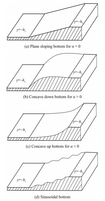Figure  2  Bottom Profiles of seabed

Download: Full-Size Img

respectively, and non-dimensional wave force on breakwater K_f and force on wall K_w are derived as

respectively. The bottom profiles used in this study are given by

In the given Eq. (36), first bottom profile is used for plane sloping bottom, concave-up and concave-down type bottom whereas second bottom profile is used for sinusoidal bottom. The parameter α used in bottom profiles determines the shape of bottom such as α = 0 renders to plane sloping bottom, α > 0 provides concave down type bottom and α < 0 corresponds to concave up type bottom. Also, second bottom profile in Eq. (36) is used for rippled type bottom, here d refers to ripple amplitude and L = sl, where l is the wavelength of rippled bottom and s denotes the number of ripples present in the bottom.

4.1   Wave trapping

In this subsection, the case of presence of impermeable wall at distance W from porous flexible breakwater is discussed. Here, effect of bottom topography and wave absorbing nature of breakwater have been studied assuming rigid impermeable wall present in front of breakwater. Thus, we present reflection coefficient K_r, wave force on breakwater K_f and wall K_w when wave interacts with porous flexible breakwater in the presence of bottom undulation.

To validate the present model, the experimental results of Krishnendu and Balaji (2020) (Figure 9(a)) concerned with the trapping of normal wave incidents are compared with the present model as shown in Figure 3(a). In this figure, continuous lines represent the present theoretical results whereas discrete points are used to show the experimental values obtained in Krishnendu and Balaji (2020). The parametric values used in this figure are α = 0, θ = 0°, W = 1 and γ_s = 1. It is to noted that When h₃/h₁ → 1 then step type bottom is converted to flat bottom and for non-dimensional flexural rigidity γ_s ≥ 1 (as in Koley et al. (2015)), breakwater works as non-flexible porous breakwater. Figure 3 is plotted to show the reflection coefficient, wave force on breakwater and wall as a function of chamber width W/λ₁. The results from Krishnendu and Balaji (2020) obtained experimentally agrees well with the present theoretical estimates as shown in Figure 3(a). To ensure the accuracy of the present model, root mean square error (RMSE) is performed. It is found that RMSE for 20% porosity is 0.05, 15% porosity is 0.024, 10% porosity is 0.024 and 5% porosity is 0.034. This RMSE values show the very good match for accuracy of the present model. It is evident from Figure 3(a) that reflection is less for higher porosity and corresponding wave force on breakwater is less whereas wave force on wall is high. It is evident from Figure 3(b) that wave force on breakwater decreases continuously with respect to non-dimensional distance between wall and porous breakwater W/λ₁. Figure 4 is plotted to illustrates the variation of reflection coefficient as a function of chamber length W/λ₁. The numerical values of parameters are taken as β₀h₁ = 1.3, α = 0, f_s = 5, ϵ_s = 0.3, s_s = 1 and d_s/h₁ = 0.05. Particularly, in Figure 4(a), the present problem is compared with the Figure 8 of Liu et al. (2007) concerning to wave trapping by thin porous breakwater in the presence of uniform bottom (h₃/h₁ = 0.99). It is found that present result matches exaclty with the plot of Liu et al. (2007) in Figure 4(a). It is to noted that for flexural rigidity γ_s = 1, breakwater becomes non flexible and act as only porous without flexibility. In Figure 4(a), dotted line represents the result of Liu et al. (2007) when breakwater is assumed to be only porous and flexibility is absent (γ_s = 1). Moreover, when water depth ratio is varying, reflection coefficient increases as depth ratio decreases and periods of oscillations reduces which leads to shift in minima. In Figure 4(b), effect of flexural rigidity γ_s is studying when length of chamber is varying on x-axis with h₃/h₁ =0.35. It is observed that least reflection is observed for γ_s =0.002 and high reflection occurs for γ_s = 0.000 2 due to much flexibility in breakwater. Hence, moderate values of flexural rigidity is preferable to attained tranquil region.

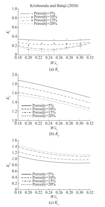Figure  3  Reflection coefficient K_r, force on breakwater K_f and force on wall K_w versus non-dimensional length W/λ₁ for different porosity with T = 2.0

Download: Full-Size Img

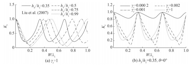Figure  4  Reflection coefficient K_r versus non-dimensional length W/λ₁ for different values of depth ratio h₃/h₁ with γ_s = 1, and for different values of flexural rigidity γ_s with h₃/h₁ = 0.35 and θ = 0°

Download: Full-Size Img

In Figure 5, reflection coefficient K_r, wave force acting on breakwater K_f and wall K_w versus non-dimensional length of varying bottom is plotted to study the effect of flexural rigidity γ_s. The numerical values of parameters used in this figure are T = 8 s, h₃/h₁ = 0.25, G = 1 + i, W/λ₁ = 0.4 and α = 1. A comparison of the present study is made in this figure with Behera et al. (2015) (Figure 3(a)) in which they analyzed wave interaction of non-flexible breakwater placed in front of an impermeable wall in the presence of step type bottom. The solid line represents the result of Behera et al. (2015) in Figure 5(a). It is observed from Figure 5(a) that higher reflection is observed for γ_s = 1 which may be due to rigid porous breakwater also, higher reflection is observed for γ_s = 0.000 02 as it allows more water to pass due to much flexibility of breakwater and reflected by impermeable wall for the smaller length of varying bottom. On the other hand, less wave force is exerted on breakwater for smaller values of varying bottom and higher wave force is noticed on wall for γ_s = 0.000 02 which is evident from Figures 5(b) and 5(c) respectively. From Figure 5, it is concluded that less reflection is observed in the case of γ_s = 0.000 1 for L/λ₁ ≥ 0.4 and more wave force exerts on breakwater which results in less wave force on the wall.

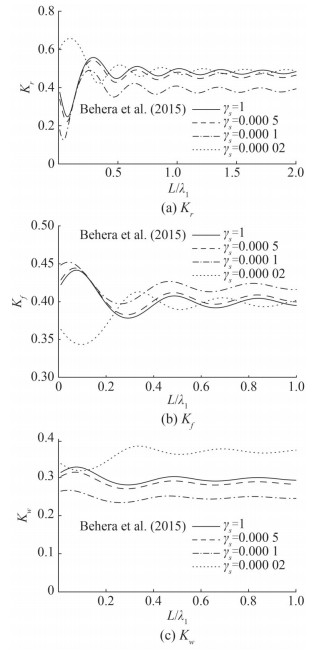Figure  5  Reflection coefficient K_r, force on breakwater K_f and force on wall K_w versus non-dimensional length L/λ₁ for different values of γ_s

Download: Full-Size Img

Figure 6 shows the variation of reflection coefficient K_r, wave force acting on breakwater K_f and wall K _w versus non-dimensional length of a varying bottom for the different bottom profile as defined in Figure 2. The numerical values of parameters are same as in Figure 5. A similar pattern is observed for concave down, plane sloping and concave up type bottom. Further, the oscillatory pattern of these bottom profiles vanishes with increasing length of varying bottom L/λ₁. Figure 6 shows that rippled bottom profile exhibits higher reflection and least waves transmitted through breakwater for the smaller length of varying bottom which causes less wave force exerting on the impermeable wall which may be a favorable situation to protect the harbor regions.

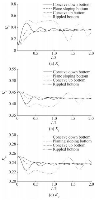Figure  6  Reflection coefficient K_r, force on breakwater K_f and force on wall K_w versus non-dimensional length L/λ₁ for different bottom profiles with flexural rigidity γ_s = EI/ρh₃⁴ = 0.02

Download: Full-Size Img

Figure 7 is plotted to examine the changes in reflection coefficient K_r, wave force acting on breakwater K _f and wall K_w for different values of depth ratio h₃/h₁ when non-dimensional wavenumber is varying on the x-axis. An oscillatory trend is observed with respect to wave number. Higher reflection occurs for flat bottom (h₃/h₁ = 0.99) and amplitude of oscillation in reflection increases as depth ratio decreases. On the other hand, Force on breakwater and wall decreases as the wavenumber increases on x-axis as observed in Figures 7(b) and (c). Hence, shallow water waves exert high wave force on the breakwater as well as on wall. Also, as the depth ratio decreases wave force on wall decreases with more minima.

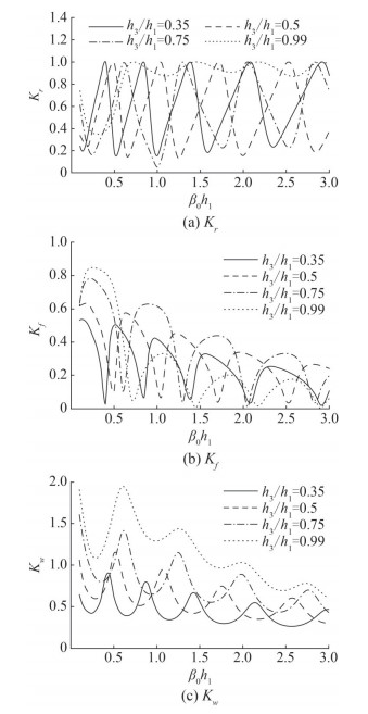Figure  7  Reflection coefficient K_r, force on breakwater K_f and force on wall K_w versus non-dimensional wavenumber β₀h₁ for different values of depth ratio h₃/h₁

Download: Full-Size Img

In Figure 8, reflection coefficient K_r, wave force acting on breakwater K_f, and wall K_w are studied as a function of the distance between breakwater and wall for different values of depth ratio h₃/h₁. These coefficients are found to be periodic with respect to the length of chamber width. Parametric values used in this figure are G = 1 + i, β₀h₁ = 1, λ_s = 0.01 and α = 0. From Figure 8(a), it is observed that the least wave is reflected for the depth ratio h₃/h₁ = 0.75 which results in high force on breakwater as in Figure 8(b). The presence of flat bottom causes high wave force on wall and the least wave force exert on the wall due to smaller values of depth ratio. It is also observed that the number of minima increases with a decrease in depth ratio. A drift towards left side in minima of wave force on wall is noticed in Figure 8(c) for decreasing depth ratio h₃/h₁.

Figure  8  Reflection coefficient K_r, force on breakwater K_f and force on wall K_w versus non-dimensional chamber length W/λ₁ for different values of depth ratio h₃/h₁

Download: Full-Size Img

Figure 9 demonstrates the effect of chamber width W/λ₁ on reflection coefficient, wave force on breakwater and wall for different values of flexural rigidity γ_s. The numerical values of parameters used in this figure are chosen as G = 1 + i, β₀h₁ = 1 and α = 0. It is observed that wave reflection and wave force on the wall is high for smaller values of flexural rigidity γ_s. Figure 9(a) illustrates that maximum reflection is achieved for certain chamber width W/λ₁ which implies minimum force attained on breakwater as in Figure 9(b). It is noted that for certain chamber width moderate values of flexural rigidity, substantial less wave force exerts on breakwater and wall.

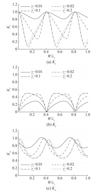Figure  9  Reflection coefficient K_r, force on breakwater K_f and force on wall K_w versus non-dimensional chamber length W/λ₁ for different values of flexural rigidity γ_s = EI/ρh₃⁴

Download: Full-Size Img

In Figure 10, reflection coefficient K_r, wave force on breakwater K_f, and wall K_w are depicted against the angle of the incident for different values of depth ratio h₃/h₁. The parameters chosen in this figure are G = 1 + i, β₀h₁ = 1, α = 0 and λ_s = 0.01. For the flat bottom (h₃/h₁ = 0.99), higher reflection occurs as shown in Figure 10(a) which causes higher wave force on the wall as observed from Figure 10(c). On the other hand, less reflection occurs for the depth ratio h₃/h₁ = 0.35 at an angle of incidence θ = 75° which implies more energy dissipation as high wave force on wall and breakwater does not exert. It is to note that full reflection is achieved for a certain angle of the incident wave at which zero wave force exerts on the breakwater. however, wave force on the wall is increasing as depth ratio h₃/h₁ is increasing for the angle of incident θ ≥ 65°.

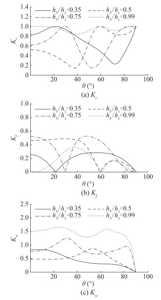Figure  10  Reflection coefficient K_r, force on breakwater K_f and force on wall K_w versus angle of incident θ for different values of depth ratio h₃/h₁

Download: Full-Size Img

Effect of different flexural rigidity on reflection coefficient K_r, wave force on breakwater K_f, and wall K_w are studied in Figure 11 when the angle of incident wave is varying on x-axis. In Figure 11, a similar pattern is observed as in Figure 10 that for a certain range of angle of incident 50° ≤ θ ≤ 70°. Figure 11(a) demonstrates that the curve of reflection coefficient shows more oscillatory for the larger values of flexural rigidity γ_s. Also, it is to note that smaller values of flexural rigidity cause more deflection which result in less wave force on barrier and high wave force on the impermeable wall as observed in Figures 11(b) and 10(c) respectively.

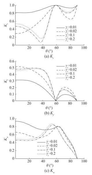Figure  11  Reflection coefficient K_r, force on breakwater K_f and force on wall K_w versus angle of incident θ° for different values of flexural rigidity γ_s = EI/ρh₃⁴

Download: Full-Size Img

In Figure 12, reflection coefficient K_r, wave force on breakwater K_f and wall K_w are illustrated with varying porous effect parameter G for different values of depth ratio h₃/h₁. The numerical value of parameters are taken as α = 0, θ = 30°, β₀h₁ = 1, λ_s = 0.01 and W/λ₁ = 1. Figure 12(a) depicts that there is large variation in reflection coefficient for porosity 0 ≤ G ≤ 2 and maximum reflection occurs for uniform bottom h₃/h₁ = 0.99. Initially, the reflection coefficient decreases sharply as G increases then it increases for larger values of G and does not alter its pattern beyond a certain value of G as shown in Figure 12(a). Smaller values of porous effect parameter (G < 2) cause less wave force is exerting on breakwater whereas force on wall is high for the uniform bottom. Figure 12(b) and (c) reveals that least wave force is acting on breakwater and wall for the depth ratio h₃/h₁ = 0.35. It is to note that wave energy is dissipated for G = 1.25 as the reflection coefficient is minimum at this point however there is no such variation in wave force on breakwater and wall. From these observations, porous effect parameter 0.5 < G < 2 may be preferable for dissipating wave energy for smaller depth ratio h₃/h₁ = 0.5 and 0.35.

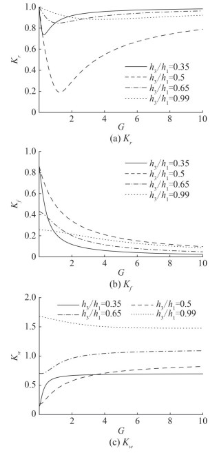Figure  12  Reflection coefficient K_r, force on breakwater K_f and force on wall K_w versus porous effect parameter G for different values of depth ratio h₃/h₁

Download: Full-Size Img

Figure 13 is plotted to show the deflection of flexible porous plate ζ/h₁ against z/h₁ for different values of flexural rigidity γ_s and porous effect parameter G when the plat is fixed at the bottom edge. Some specific amount of parameters are fixed as h₃/h₁ = 0.5, W/λ₁ = 1, α = 0, θ = 30° and β₀h₁ = 1. From Figure 13(a), the plate is much deflected when flexibility γ_s is added to the breakwater which is an obvious phenomenon. Also for rigid breakwater G = 0, deflection is high as compared to porous flexible breakwater since it does not allow transmission of water as observed in Figure 13(b) which causes high wave force on breakwater as observed in Figure 12(b).

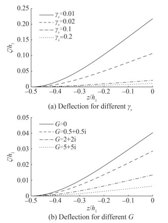Figure  13  Plate deflection ζ/h₁ versus z/h₁ for different values of γ_s with G = 1 + i and G with γ_s = 0.1

Download: Full-Size Img

4.2   Wave scattering

In coastal regions or marinas, it is desirable to maintain healthy ecosystem and make harbour free from stagnating pollution. It is assumed that there are no fixed boundaries at far field, hence, in this subsection, we present scattering of waves by flexible porous breakwater in the presence of uneven bottom. In this case, a part of wave energy will be dissipated and some will be transmitted to lee side of breakwater. Thus, in this view point, we study reflection coefficient K_r and transmission coefficient K_t and wave force on wall K_f.

Figure 14 demonstrates the influence of various bottom profiles with varying horizontal bottom length L/λ₁ on reflection, transmission and wave force on breakwater. The used parameters to plot these graph are as h₃/h₁ = 0.25, γ_s = 0.02, G = 1 + i and T = 8 s. The observation received in this plot is similar to the case of trapping of waves as in Figure 6. The result demonstrates that each type of bottom shows higher reflection and oscillatory pattern for smaller length of bottom and curves variation diminish as its length increases except for the case of rippled bottom. It is observed from Figure 14 that most of the wave energy is reflecting due to presence of rippled bottom for small length of varying bottom which leads to least transmission and hence least hydrodynamic force exerts on flexible breakwater.

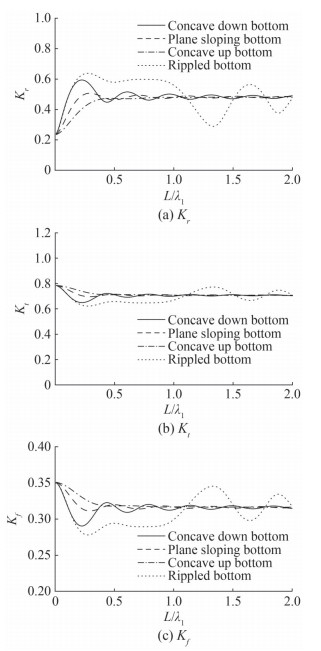Figure  14  Reflection coefficient K_r, transmission coefficient K_t and force on breakwater K_f versus length of varying bottom L/λ₁ for different bottom profiles

Download: Full-Size Img

Further, to analyze the effect of depth ratio h₃/h₁ and flexural rigidity γ_s of flexible porous breakwater on Bragg reflection which takes place in the presence of sinusoidal bottom. The phenomenon of Bragg resonance can be found in several articles such as Dalrymple and Kirby (1986), Tabssum et al. (2020) in the presence of structures. The ideal condition for Bragg resonance is 2l/λ₁ = 1 at which reflection enhances significantly. In the present article, reflection and transmission coefficients K_r, K_t and wave load on porous breakwater K_f are studied in Figure 15 and Figure 16 as a function of frequency parameter 2l/λ₁.

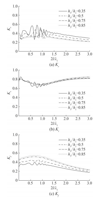Figure  15  Reflection coefficient K_r, transmission coefficient K_t and force on breakwater K_f versus 2l/λ₁ for different values of depth ratio h₃/h₁

Download: Full-Size Img

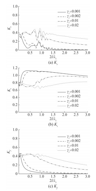Figure  16  Reflection coefficient K_r, transmission coefficient K_t and force on breakwater K_f versus 2l/λ₁ for different values of flexural rigidity γ_s

Download: Full-Size Img

Figure 15 is presented to show the effect of depth ratio h₃/h₁ on Bragg scattering coefficients. The fixed parameters for this figure are as G = 1 + i, γ_s = 0.02, L₁ = 10, s = 6, l = 6.4 and d = 0.08. Figure 15(a) reveals that more Bragg resonance is pronounced near 2l/λ₁ = 0.75 and reflection is high for depth ratio h₃/h₁ = 0.35. Moreover, reflection coefficient decreases as depth ratio increases and resonance peak shifts towards right. It is seen that least transmission occurs at 2l/λ₁ = 0.75 which may be favourable condition for creating calm zone near harbour region but variation with respect to different depth ratio is negligible. However, significant variation is noticed with respect to depth ratio. Least hydrodynamic force is exerting on porous flexible breakwater for depth ratio h₃/h₁ = 0.35.

Figure 16 shows the influence of flexural rigidity γ_s on Bragg scattering coefficients. The parameters used to plot this figure are same as in Figure 15. From Figure 16(a), it exposes that least reflection is pronounced at 2l/λ₁ = 0.9 for smaller values of flexural rigidity which leads to higher transmission and less wave force as in Figures 16(b) and (c) respectively. It is observed that higher wave energy dissipation occurs for larger values of frequency parameter as zero reflection and wave force on breakwater is observed whereas transmission is less less for γ_s = 0.001 and 0.002.

In Figure 17, deflection of the flexible porous breakwater is shown for different values of flexural rigidity γ_s = EI/ρhh₁⁴ and porous effect parameter G. The parameters used in this plot are β₀h₁ = 1, α = 0, γ_s = 0.1 and G = 1 + i. From Figure 17(a), plate deflection is observed high for small values of flexural rigidity γ_s = 0.01 and less deflection for higher values as noticed in Figure 13(a). Deflection decreases as flexural rigidity increases. In Figure 17(b), highest deflection occurs for impermeable breakwater for G = 0. However, deflection is less as compare to the case of trapping in Figure 13 which may be due to absence of impermeable wall.

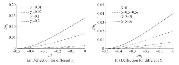Figure  17  Plate deflection for different values of flexural rigidity γ_s = EI/ρhh₁⁴ and porous effect parameter G

Download: Full-Size Img

5   Conclusions

In the present study, the effect of bottom variation on the trapping and scattering of obliquely incident waves is analyzed using a flexible porous breakwater. The study is carried out within the framework of linear water wave theory, and Darcy's law is used to model the flow past the porous breakwater. To solve the physical problem, an eigenfunction expansion in the region of uniform bottom is coupled with the mild-slope equation for step-type bottom topography. The system of equations is obtained by imposing suitable boundary conditions at the interface, and mass-conserving jump conditions are applied at the slope discontinuities on the bottom edge. The present theoretical model is compared with the result of Krishnendu and Balaji (2020) in less general case of porous breakwater in the presence of uniform bottom. Further, the results are validated with the plot of Behera et al. (2015) and Liu et al. (2007) in a limiting case.

The study reveals that wave reflection increases and minima drags towards left as depth ratio decreases. Additionaly, minimum reflection occurs for flexural rigidity γ_s = 0.002. Further, the breakwater reflects less wave energy and exerts less wave force on the wall for intermediate values of the flexural rigidity γ_s. A large variation is observed for smaller values of the varying lengths of the bottom. However, a rippled type bottom profile may be more preferable for creating a tranquil environment, as it allows for more reflection and leads to the least force on the breakwater and wall for smaller lengths of varying bottom (L/λ₁ < 1.25). The oscillatory behavior of the reflection coefficient increases as the depth ratio decreases, and the amplitude of oscillation reduces as the non-dimensional wavenumber increases. For a particular distance between the breakwater and wall, and angle of incidence, negligible force is acting on the breakwater. It is observed that smaller values of the flexural rigidity of the breakwater result in less wave force on the breakwater and higher force on the wall for an angle of incidence θ > 60°. Moreover, due to the presence of a step-type bottom, complete reflection occurs for large values of G, and the force on the breakwater diminishes, resulting in the least force exerted on the wall. Plate deflection is more pronounced for smaller values of the porous effect parameter.

In the case of wave scattering, higher reflection is noticed for a rippled bottom with a smaller length of varying bottom. A smaller depth ratio allows for higher reflection and least transmission. Bragg resonance is pronounced at 2l/λ₁ = 0.75, which may be a favorable case for a tranquil region near the harbor. Wave energy dissipation is higher for larger frequency parameters. Less deflection is observed in the case of scattering compared to wave trapping.