1   Introduction

Aquaculture vessels, a new type of aquaculture equipment for deep-sea fishery, can provide a suitable environment for the breeding of fish in tanks at sea (Guo et al., 2020; Xue et al., 2022). Given the particular function of aquaculture tanks, the seawater they contain can severely corrode their bulkhead to jeopardize their structural safety. The sloshing load of aquaculture water in tanks caused by hull motion also has a great influence on their structural safety (Cui et al., 2022; Hui et al., 2022).

Although numerous studies have investigated the effects of sloshing load on structural strength, most focused on ships carrying liquid cargo, such as oil tankers and LNG carriers (Dumitrache and Deleanu, 2020; Park et al., 2021). The empirical formula for calculating the strength of tank structures in the presence of a sloshing load has been proposed by the classification societies of various countries. Among the proposed methods, the simplest involves calculating the sloshing load on the basis of an empirical formula and using it to evaluate structural strength (Zhang, 2018). Current studies in the effects of sloshing load on structural strength focus on direct and effective numerical methods. For example, Park et al. (2023) investigated the dynamic responses of an LNG cargo containment system by using the triangular impulse response function. Yun et al. (2020) developed two-way cosimulation technology on the basis of DualSPHysics and RecurDyn and applied it to solve the problem of sloshing inside a tank connected to the upper plate of a six-DOF platform. They investigated the effects of the dynamic load of fluid on structural safety. Lee and Paik (2021) examined nonlinear impact structural response characteristics under sloshing impact loads by utilizing a nonlinear finite element ANSYS/LS-DYNA method. Dumitrache and Deleanu (2020) studied the influence of tank sloshing caused by hull motion on the strength of ballast tank structures and found that the cyclic mechanical stress caused by sloshing can produce fatigue stresses in the welded joints of hulls. Hwang and Lee (2021) extended the velocity of sloshing flow (calculated by CFD) to the real scale and applied it in a local two-way fluid–structure interaction analysis of the load conditions and structural response of LNGs.

Although numerous simplified corrosion models have been proposed to study hull corrosion in a specific environment or specific steel, these models have certain limitations (Ivošević et al., 2017; Zayed et al., 2018; Yao et al., 2018). COMSOL Multiphysics software has emerged as a potential tool for analyzing corrosion and variation in different parameters. For example, Iwamoto (2019) conducted validation by comparing corrosion simulation results from COMSOL Multiphysics and experimental results obtained by using the mock-up sheet pile model. They verified that the potential distributions obtained from experimental results were consistent with those acquired through simulations. Gupta et al. (2022) investigated the galvanic corrosion behavior of rivet-joint systems by using time-dependent simulation with the help of COMSOL Multiphysics software. In addition, Prajapati et al. (2022), Chalgham et al. (2019), and Feng et al. (2022) conducted corrosion simulation calculations by using COSMOL Multiphysics software and achieved satisfactory results.

In some special environments, corrosion has a great effect on the strength of ship structures. Vu and Dong (2020) introduced a probabilistic model to estimate the rate of corrosion and assessed the effects of corrosion in flanges and webs on the cross-sectional properties and ultimate strength of bulk carriers. Georgiadis and Samuelides (2019) reassessed ultimate strength by updating the time-variant corrosion model and exploiting on-site observations from thickness measurement reports within the framework of Bayesian updates. Given that aquaculture vessels are a new type of deep-sea aquaculture equipment, their working environment and structural form are considerably different from those of ordinary vessels. No relevant structural rules are currently available for the strength assessment of aquaculture vessels. In addition, the conventional method for calculating corrosion allowance in strength assessment involves using the empirical values recommended by classification societies. However, during operation, the proportion of the area of contact between seawater or aquaculture water and the inner or outer surfaces of ships is large. In addition to the conventional components of seawater, aquaculture water contains substances that may cause marine steel to corrode. These substances include feed, fungicides, nutrients, and fish excrement. Various factors indicate that the problem of corrosion in aquaculture vessels is more serious than that in ordinary vessels (Feng et al., 2022). Therefore, the corrosion allowance recommended in the rules for ordinary vessels may be unsuitable for aquaculture vessels.

In this study, the working characteristics of aquaculture vessels were considered, and a model for analyzing the structure of aquaculture tanks was established. The corrosion simulation of aquaculture tanks based on multiphysical field coupling analysis was proposed by considering the working environment of aquaculture vessels. Wave and sloshing loads were calculated on the basis of potential flow theory and computational fluid dynamics (CFD), respectively. Furthermore, the influence of corrosion allowance and sloshing load calculated by different calculation methods on aquaculture structural responses was analyzed. Finally, a coupling direct calculation method for the structural responses of aquaculture tanks was proposed and used to calculate structural responses.

2   Calculation model

The aquaculture vessel used in this study is equipped with 16 aquaculture tanks in two rows along the ship, as shown in Figure 1. The internal structure of the tanks is depicted in Figure 2. The vessel conducts aquaculture operations in the Yellow Sea and East China Sea. The main dimensions of the vessel and tank are given in Table 1.

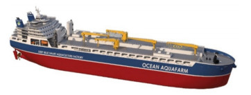Figure  1  Aquaculture vessel

Download: Full-Size Img

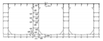Figure  2  Structural layout of aquaculture tanks

Download: Full-Size Img

3   Multiphysical field coupled simulation calculation of corrosion

3.1   Basic principle

3.1.1   Electrode reaction

Corrosion is a special redox reaction. During the corrosion of aquaculture tanks, steel is in contact with seawater. Given that water molecules are polar, they strongly attract the iron ions that are in direct contact with seawater. The relevant chemical reaction is as follows:

where Fe is the iron atom, Fe²⁺ is the ferrous ion, M is the solid phase, and Sol is the liquid phase.

The concentration of ferrous ions in the water increases with the progression of corrosion. Ferrous ions accumulate near the interfacial region to form a high concentration gradient, which in turn causes them to react to form iron atoms attached to the metal phase. The chemical reaction is as follows:

The reactions represented by the above two equations occur simultaneously in corrosion as follows:

Gibbs' free energy is the basis for judging whether the corrosion reaction can proceed. Whether the redox reaction can occur spontaneously can be determined in accordance with the following formula:

where ΔG is the change in Gibbs' free energy, A and B are reactants, C and D are products of the reaction, ν is the stoichiometric number of the substance, and μ is its electrochemical potential.

When ΔG < 0, the reaction can occur spontaneously.

When ΔG > 0, the reaction cannot occur spontaneously.

When ΔG = 0, the reaction reaches a state of chemical equilibrium, and the reaction rates in the forward and reverse directions are equal.

When the reaction has been determined to be capable of occurring spontaneously during corrosion, whether the reaction proceeds in the forward or reverse direction at a certain point in time must also be determined. The product of the stoichiometric number and chemical potential during the reaction is divided by the product of the charge in the reactive ion and Faraday constant, which is called the Galvani potential and is represented by φ:

When a redox reaction reaches equilibrium, the Galvani potential calculated in accordance with the above formula is called the equilibrium potential of the reaction and is represented by φ_e.

When φ_e > φ, the reaction proceeds in the positive direction.

When φ_e < φ, the reaction proceeds in the negative direction.

When φ_e = φ, the reaction reaches a state of dynamic equilibrium.

3.1.2   Corrosion mathematical model

In corrosion simulation, corrosion needs to satisfy the mass transfer conservation, charge conservation, and local electric neutrality equations, as shown in Equations (6), (7), and (8), respectively:

where c is substance concentration, i is the type of substance, and t is the time item. The flux N is calculated as

where − D∇c_i is the diffusion term, u_m is the electromigration number, z_iu_{m, i}Fc_i∇φ_l is the electric migration item, and c_iu is the convective term.

The net current in the electrolyte is described by using the total material flux

The charge conservation and local electric neutrality equations are

3.2   Corrosion model

We believe that the corrosion of aquaculture tanks is a coupling problem of multiple physical fields. In accordance with the theory of corrosion electrochemistry, corrosion often occurs at sharp points, corners, or weld seams wherein surface geometry is severely discontinuous, given the presence of strong electrolytes in seawater. These locations exhibit particularly severe corrosion due to their high corrosion current density. However, as corrosion occurs, the morphology of these positions gradually changes, and sharp positions may be passivated, leading to a decrease in corrosion current density and a change in structural corrosion characteristics. From the perspective of the overall structure, a high density of corrosion current is generated at the new location. This situation indicates that the corrosion location has changed. In addition, in actual corrosion simulation analysis, the vertical gradient change of oxygen concentration should be considered, and oxygen concentration is another important factor affecting corrosion. The corrosion of aquaculture tanks can be seen as a coupling problem of multiple physical fields. Such a problem should at least include the coupling of solid structure, distribution of corrosion electrochemical parameters, and distribution of physical parameters (such as oxygen concentration).

Corrosion in different regions of aquaculture tanks differs. In accordance with the characteristics of the seawater environment of aquaculture tanks, corrosion regions can be divided into splash, main, and sediment corrosion regions (Figure 3). A real-scale finite element model was established in accordance with the size of the aquaculture tank in the multiphysics coupling analysis software COMSOL Multiphysics (Figure 4). The structures near the waterline, hatch corners, and weld seams are refined on the basis of the coarse grid.

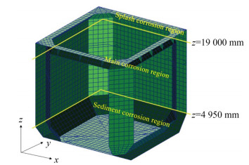Figure  3  Corrosion regions in an aquaculture tank

Download: Full-Size Img

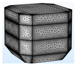Figure  4  Finite element model of an aquaculture tank in COMSOL

Download: Full-Size Img

3.3   Hydrological conditions of aquaculture tanks

The hydrological condition and electrochemical parameters of aquaculture tanks are key parameters affecting the results of corrosion simulation. The parameters of the hydrological conditions and electrochemical parameters in accordance with the species of fish being bred in the aquaculture vessel are shown in Tables 2 and 3.

3.4   Calculations in corrosion simulation

The lifecycle of aquaculture vessels is 20 years. Corrosion simulations were conducted for the 20-year lifecycle of the vessel studied in this work. COMSOL Multiphysics analysis commercial software was used to simulate tank corrosion in accordance with the relevant theory of the electrochemistry of corrosion and in consideration of the hydrological conditions of the aquaculture tank and corresponding anticorrosion measurement (epoxy paint as an anticorrosive coating). The corrosion thicknesses of the tank structures for 20 years were calculated. The results are shown in Figures 5 and 6.

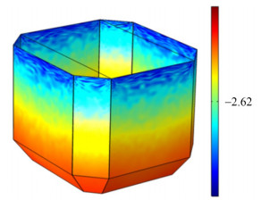Figure  5  Cloud image of corrosion thickness in the aquaculture tank

Download: Full-Size Img

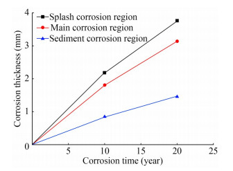Figure  6  Simulation of corrosion thickness in aquaculture tanks

Download: Full-Size Img

Figure 5 is the cloud image of the corrosion thickness of the aquaculture tank. The most severe corrosion occurs in the bulkhead near the waterline, that is, in the splash corrosion region. Figure 6 shows that over the 20-year period, the maximum corrosion thickness in the splash corrosion region is 3.79 mm. The structures in this region are near the liquid surface, which is humid all year round. The air around the structures contains a large amount of chloride, which exerts a strong decomposing effect on the oxide film on the surface of the aquaculture tank, aggravating the effect of corrosion and causing the most serious corrosion in this region. Corrosion in the sediment corrosion region over 20 years is relatively small, with a maximum thickness of 1.46 mm. Among the regions, the sediment corrosion region is the farthest from the water surface. Seawater has a low oxygen concentration. Therefore, galvanic corrosion mainly occurs in this region. The welding materials used at the weld of the plate are different from the materials of the hull plate. They are in direct contact with each other, creating conditions for the occurrence of galvanic corrosion. The corrosion thickness of the structure in the main corrosion region is between those in the splash and sediment corrosion regions. In this region, the maximum thickness is 3.16 mm over 20 years. The structure of the main corrosion region is located below the waterline and is completely immersed in seawater. Seawater acts as a good conductor of ions to create conditions for corrosion. At the same time, because this region contains abundant oxygen, corrosion occurs in this region. However, given that the oxygen content in the water in the main corrosion region is not as high as that in the splash corrosion region, the degree of corrosion in this region is smaller than that in the splash corrosion region. The cloud image of the corrosion thickness in the main corrosion region illustrates that with the increase in depth, corrosion thickness gradually decreases because the concentration of oxygen in seawater varies with depth.

The structure of aquaculture vessels is similar to that of double-hulled oil tankers. Currently, the strength assessment of the aquaculture tank is usually conducted by referring to the relevant classification society's rules for double-hulled oil tankers, such as the China Classification Society's (CCS) Rules for the Classification of Sea-going Steel Ships (Han et al. 2020). The comparison between the corrosion allowance specified in CCS rules and the simulation results of corrosion is shown in Table 4 (provisions for corrosion allowance are specified in Part 9, Chapter 3, Section 1 in Rules for the Classification of Sea-going Steel Ships).

The provisions for the corrosion allowance of oil tankers in CCS rules are based on empirical values. Given that the environment in aquaculture tanks is more corrosive than that in oil tanks, the simulated results of 20 years are larger than the corrosion allowances given in CCS rules. The literature states that the average corrosion rate of a steel structure in seawater is 0.11–0.14 mm/year and that the local corrosion rate can reach as high as 0.6 mm/year (Lan et al. 2012). In the simulation of corrosion over 20 years, the average thickness of corrosion in the aquaculture tank was 2.80 mm, and the average corrosion rate was 0.139 mm/year, which is consistent with the measurement results in the references. We also compared the measured corrosion rates of 441 KW (600 PS) steel fishing vessels built by the Dalian Ocean Fisheries Group Shipyard in Liaoning Province, China (Qu et al. 1988). These fishing vessels operate in the East China Sea and the Yellow Sea, consistent with the working status and environment of the aquaculture vessel studied in this work. The average corrosion rate of the steel fishing vessel fish tank is 0.143 mm/year, which is close to the simulation result of 0.139 mm/year. Therefore, simulating the corrosion of an aquaculture water tank through multiphysical field coupling analysis is correct.

4   Calculation of design loads

4.1   Wave load

4.1.1   Mathematical model

In accordance with three-dimensional linear potential flow theory, the total velocity potential in flow fields is

where −Ux is the uniform flow, ϕ_s (x, y, z) is the wave-making potential, and ϕ_T (x, y, z)e^iωt represents the unsteady velocity potential of waves. The unsteady velocity potential can be decomposed into the following form:

where ϕ_I (x, y, z) is the incidence potential, ϕ_D (x, y, z) is the diffraction potential, and ϕ_R (x, y, z) represents the radiation potential.

In accordance with the theory of rigid body dynamics, the motion equation of ships in regular waves can be expressed as

{F^S(t)} represents the hydrostatic load, which can be expressed as

where P_S (x, y, z, t) is the hydrostatic pressure caused by ship motion, and [C] is the hydrostatic coefficient.

{F^D(t)} is the hydrodynamic load, which can be expressed as

where {F_I(t)}, {F_D(t)}, and {F_R(t)} represent the incident, diffraction, and radiation wave forces, respectively. On the basis of plane wave theory and the Bernoulli equation, the pressure distribution is obtained by deriving the incident, diffraction, and radiation potentials. The pressure distribution on the wet surface of the ship is integrated to obtain incident, radiation and diffraction forces. The expressions for incident, radiation and diffraction forces are

Subsequently, the linear frequency domain rigid body dynamics equation for ship motion in regular waves is

where [M] is the hull mass matrix; [A] is the additional mass matrix of the hull; {η(t)} represents the hull motion with six degrees of freedom; [B] is the fluid damping coefficient; [C] is the hydrostatic coefficient; {f(t)} is the wave interference face; and {f}e^iωt is the form after the spatiotemporal separation of wave interference forces.

4.1.2   Design wave method

The loads for structural analysis were calculated by using the design wave method. The design wave expression is

where A is the amplitude of the design wave; ω is the frequency; ε_m is the phase corresponding to the maximum value of the load transfer function; and the sum of ε_m and ε is equal to 0° or 180°, which correspond to the sagging and hogging states, respectively.

The wave direction and frequency corresponding to the maximum value of the response amplitude operators of the main control load are the design wave direction and frequency. The design wave amplitude is calculated by using

where the design value of the main control load is calculated through long-term analysis.

4.1.3   Wave load calculation

The wave loads of the aquaculture vessel were calculated by using the commercial software COMPASS-WALCS-Basic on the basis of 3-D potential flow theory. The stats of the East China Sea and Yellow Sea, wherein the aquaculture vessel operates, were used in the calculation of the design loads. The exceeding probability was determined in accordance with the number of waves encountered during a 20-year service period. Given that the sloshing load is an important load acting on the tank structures, it was selected as the main control load in addition to the vertical bending moment. Tank sloshing is mainly excited by the roll motion of the vessel. Therefore, roll motion was used as the main control load instead of sloshing load in design load calculation.

By using parameterized modeling methods, the hull surface mesh is divided on the basis of hull shape lines. The hydrodynamic mesh of the hull surface is shown in Figure 7 (a). The floating state is adjusted in accordance with the mass distribution of the hull, and the obtained wet surface mesh and calculation sections are shown in Figure 7 (b).

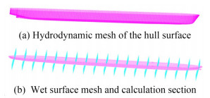Figure  7  Hydrodynamic calculation model

Download: Full-Size Img

Then, the long-term prediction of wave loads was conducted, and the long-term prediction values of the main control loads are listed in Table 6. The parameters of the design waves are shown in Table 7.

4.2   Calculation of sloshing loads

4.2.1   Mathematical model

The incompressible viscous flows of two immiscible fluids, i.e., air and water, are governed by Reynolds-averaged Navier–Stokes equations (Equations (1) and (2)).

where ρ is the fluid density, ρ = 1 024 kg/m; v is the mean velocity; p is the mean pressure; I is the identity tensor; T is the mean viscous stress tensor; and f_b is the resultant of the body forces. The additional term (T_RANS) is the stress tensor, which has the following definition:

where k is the turbulent kinetic energy.

We use the standard k − ε SST model to simulate turbulent flow. The transport equations for kinetic energy k and specific dissipation rate ω are

where μ is the turbulent kinetic energy; σ_k and σ_ω are the model coefficients, σ_k = 0.5 and σ_ω = 0.5; and P_k and P_ω are production terms. f_β* is the free-shear modification factor, f_β* = 1; f_β is the vortex-stretching modification factor, f_β = 1;k₀ and ω₀ are the ambient turbulence values that counteract turbulence decay.

4.2.2   Calculation of sloshing loads

The tank sloshing load was calculated by using the CFD software STAR-CCM+. Pitch motion was considered in the structural analysis because it can also induce sloshing in aquaculture tanks under head sea conditions. High sloshing amplitudes can be expected when the frequency of tank motion is close to the natural frequency of a fluid. For a given rectangular prismatic tank, the natural frequencies of the fluid, depending on the fill depth, are given by

where L is the tank width, d is the water depth, and n is the mode number. In accordance with Equation (28), the natural frequency of the tank is 1.31 rad/s. The natural frequency of ship roll motion is 0.6 rad/s. Given that the motion response of the ship is very small at 1.31 rad/s, the tank response caused by ship motion will not occur. Therefore, the calculation in this study ignores tank resonance.

Roll and pitch motions were regarded as the external excitation of the sloshing in the tank, and the expression of the motions in the numerical simulation is

where A and ω are the amplitude and frequency of external excitation, respectively.

On the basis of the design wave parameters in Table 7, the amplitudes of the pitch and roll motions were calculated by using COMPASS-WALCS-Basic. Subsequently, the results, as shown in Table 9, were input into the numerical simulation of tank sloshing.

The CAD software CATIA V5 was used to generate the geometric model of the aquaculture tank. The geometric model was then imported into STAR-CCM+. The top of the tank was set as a pressure outlet boundary, and the rest of the walls were set with wall boundary conditions. The standard k − ε SST model was used to simulate turbulent flow. Grid convergence analysis was performed, and the size of grids used for calculation was determined to be 0.1 m (see Figure 9). The cloud image of the sloshing pressure calculated at 1/4 T₁ under WC06-1 is shown in Figure 10 (a), and the time history curve of sloshing dynamic pressure is provided in Figure 10 (b). (T₁ is the period of the roll motion under the WC06-1 working condition).

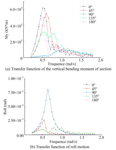Figure  8  Amplitude frequency response results

Download: Full-Size Img

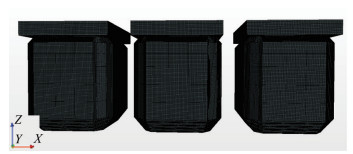Figure  9  STAR-CCM+ computational grid model

Download: Full-Size Img

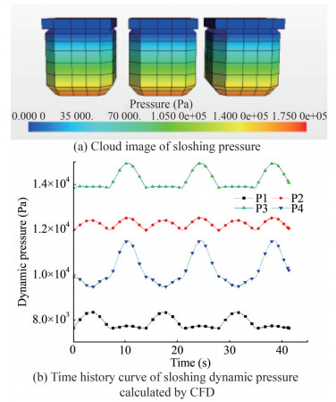Figure  10  Cloud image and time history curve of sloshing pressure

Download: Full-Size Img

Sloshing pressure was calculated in accordance with the provisions for sloshing pressure in Part 9, Chapter 4, Section 6 in Rules for the Classification of Sea-going Steel Ships to compare the CFD and CCS rule methods. Comparison results are shown in Table 10. The dynamic pressure calculated on the basis of CCS rules is greater than the dynamic pressure calculated on the basis of CFD.

5   Structural response calculation

5.1   Finite element calculation model

Part 9, Chapter 7, Section 2 in Rules for the Classification of Sea-going Steel Ships stipulates the selection range of calculation cabins. Therefore, tanks No. 5–10 were selected as targets in the structural response calculation. The finite element model in Patran is shown in Figure 11.

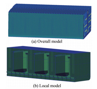Figure  11  Finite element model of the aquaculture tank

Download: Full-Size Img

5.2   Results and discussion

The commercial FEA software Patran/Nastran was used to calculate the structural response of the tank model. The direct calculation loads in Section 4.1. are used for wave loads in all calculation conditions. The calculation working conditions are shown in Table 8. In the analysis of results, the tank structures were divided into several typical parts, such as the bottom plate, bottom inclined plate, transverse bulkhead, and longitudinal bulkhead.

5.2.1   Effect of corrosion allowance

The corrosion allowance in WC01-1, WC01-2, WC02-1, and WC02-2 were calculated in accordance with CCS rules. The calculation results for structural stress are shown in Table 11. The corrosion allowance in W03-1, WC03-2, WC04-1, and WC04-2 was calculated by the multiphysical field coupling analysis described in Section 3, and the calculation results of structural stress are shown in Table 12. Comparing the stress under the same wave loads and sloshing load working conditions revealed that the stresses of the bottom plate under WC03-1 and WC03-2 are 4.8% and 4.5% larger than those under WC01-1 and WC01-2, respectively. Similarly, the stresses of the bottom inclined plate under WC03-1 and WC03-2 are 0.9% and 0.7% larger than those under WC01-1 and WC01-2, respectively. The structural stresses calculated on the basis of the simulated corrosion allowance are similar to those calculated on the basis of the corrosion allowance stipulated in CCS rules because the bottom plate and bottom inclined plate are located in the sediment corrosion region, and the corrosion simulation calculation value of this part is close to the value stated in CCS rules. The stresses of the transverse bulkhead under WC04-1 and WC04-2 are 17.4% and 18.0% larger than those under WC02-1 and WC02-2, respectively. The stresses of the longitudinal bulkhead under WC04-1 and WC04-2 are 11.7% and 11.0% larger than those under WC02-1 and WC02-2, respectively. The results of structural stress calculated by using two kinds of corrosion allowances differ greatly at the transverse and longitudinal bulkheads because the corrosion allowance of transverse and longitudinal bulkheads in the splash and the main corrosion regions calculated through simulation is quite different from the values in CCS rules. In view of the overall structure, the structural stress calculated by the corrosion simulation value is approximately 8% larger than the corrosion value in the rules.

5.2.2   Effect of sloshing load

The sloshing loads in WC05-1, WC05-2, WC06-1, and WC06-2 were calculated by using the CFD method introduced in Section 4.2 and imported into Patran/Nastran by using the Patran Command Language interface for structural response calculation. The calculation results for structural stress are shown in Table 13. Comparing the stress under the same wave loads and corrosion allowance working conditions revealed that the stress of the bottom inclined plate under WC05-1 and WC05-2 are 18.6% and 22.0% smaller than those under WC01-1 and WC01-2, respectively. Similarly, the stress of the bottom plate under WC06-1 and WC06-2 are 37.6% and 37.4% smaller than those under WC02-1 and WC02-2, respectively. The structural stress of the sloshing load calculated by CFD is smaller than that calculated in accordance with CCS rules because, as discussed in Section 4.2, the sloshing load calculated by CFD is less than that calculated by the empirical formula given by CCS rules.

5.2.3   Effect of coupling direct calculation

Coupling direct calculation was applied to calculate structural responses in this study. In this method, corrosion allowance was calculated by the multiphysical coupling field method, and the sloshing load was calculated by the CFD method. The process of coupling direct calculation is illustrated in Figure 12. The calculation results are shown in Table 14. Comparison with the structural stress results calculated on the basis of CCS rules in Table 11 shows that the stresses of the bottom inclined plate under WC07-1 and WC07-2 are 18.9% and 19.6% smaller than those under WC01-1 and WC01-2, respectively. The stresses of the bottom plate under WC08-1 and WC08-2 are 33.8% and 33.2% smaller than those under WC02-1 and WC02-2, respectively. Structural stress based on the coupling direct calculation method is significantly smaller than that based on the conventional method. In other words, if the conventional method is used to calculate the structural response of the aquaculture tank and the structural response results are used to check the structural strength, then the check results may be too conservative. This situation may easily lead to structural redundancy. Therefore, compared with the conventional method, the proposed coupling direct calculation method for the structural response calculation of aquaculture tanks can better combine the specific environment of aquaculture tanks and provide more accurate calculation results.

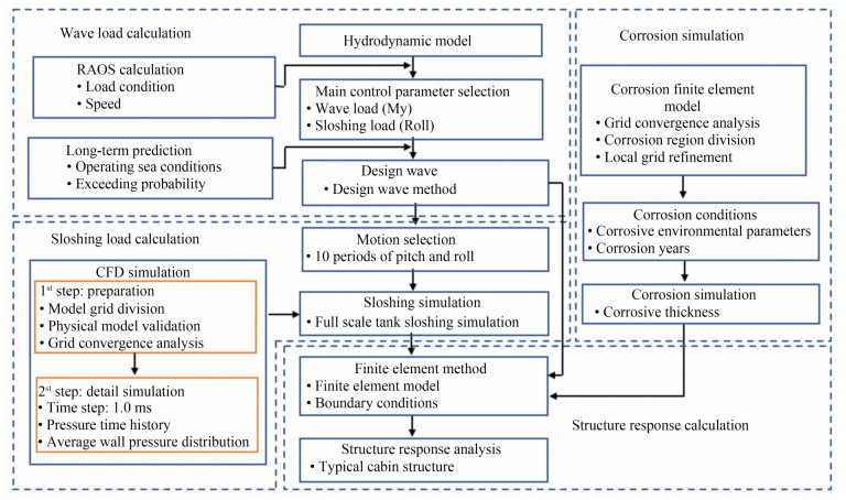Figure  12  Coupling direct calculation

Download: Full-Size Img

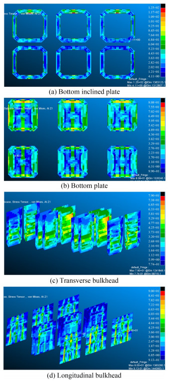Figure  13  Cloud image of structural stress in the sagging state under the working condition LC04

Download: Full-Size Img

At the same time, compared with the structural stress calculation results under different main control loads in Table 14, the structural stress calculated on the basis of sloshing load is significantly larger than that calculated on the basis of wave load. The stresses of the bottom inclined plate under WC08-1 and WC08-2 are 26.0% and 11.5% larger than those under WC07-1 and WC07-2, respectively. The stresses of the bottom plate under WC08-1 and WC08-2 are 15.7% and 13.4% larger than those under WC07-1 and WC07-2, respectively. We can conclude that due to the special sloshing environment and tank structure of aquaculture vessels, the sloshing load should be considered when determining the main control load for strength checks.

6   Conclusions

The corrosion of a 100 000-ton aquaculture vessel in the aquaculture environment was simulated through multiphysical field coupling analysis. The wave and sloshing loads on the aquaculture vessel were calculated on the basis of potential flow theory and the CFD method, respectively. The design load was determined on the basis of different main control parameters. The influence of different calculation methods for corrosion allowance and sloshing loads on aquaculture structural stress was analyzed. Finally, a coupling direct calculation method for the structural response of aquaculture tanks was proposed, and the structural response was calculated. The main conclusions are as follows:

(1) The corrosion characteristics of aquaculture tanks are considerably different from those of ordinary ships, given their special aquaculture environment. The corrosion calculated through multiphysical field coupling analysis is closer to measurements than that calculated by using the traditional empirical formula.

(2) Sloshing load has an important effect on the structure of aquaculture tanks. In the determination of the design load, the working condition under which the sloshing load is the main control parameter should be considered in addition to the wave load, which is considered the main control parameter in conventional practice.

(3) The proposed coupling direct calculation method for the structural response calculation of aquaculture tanks can well combine the specific environment of aquaculture tanks and provide highly accurate calculation results.