1   Introduction

The Earth's ocean area significantly exceeds its land area, and the ocean contains abundant resources. Therefore, countries worldwide have increasingly focused on ocean development and protection. Owing to the complexity of ocean background noises and the non-linear, non-Gaussian, and non-stationary properties of underwater acoustic signals, the detection and mitigation of noise in underwater acoustic signals are vital (Tucker et al., 2016; Li et al., 2018b). Therefore, the research and application of underwater acoustic signal denoising methods are of great significance in the underwater acoustic field.

Matched filters have been widely used in the past (Islam and Chong, 2014). These filters effectively utilize the differences between signals and noise distributions and use specific filters that match the frequency characteristics of both signals to achieve noise reduction. However, the use of matched filters for denoising non-stationary signals has limitations. Moreover, wavelet-based methods are used for denoising signals, but these methods require pre-selection of basis functions, and their effectiveness is not ideal as the frequency bands of useful signals and noise overlap (Yue et al., 2019; Wess and Dixon, 1997). Huang et al. (1998) proposed a new signal decomposition method named empirical mode decomposition (EMD). EMD can decompose a signal into high-to-low components and serve as an adaptive signal processing technique suitable for non-linear and non-stationary processes. This method was significantly used for signal denoising (Cui and Chen, 2015; Lu et al., 2016). However, EMD is susceptible to mode mixing, which leads to signal loss and affects signal processing. To solve this issue, Wu and Huang (2011) improved EMD and proposed a modified signal decomposition method named ensemble empirical mode decomposition (EEMD). EEMD incorporates the properties of EMD, adaptively processes non-linear and non-stationary signals, and effectively mitigates mode mixing.

Recently, numerous denoising methods based on EEMD and its improved algorithms have been widely used in different fields. Zhao et al. (2011) used the EEMD algorithm for denoising Electrocardiogram (ECG) in the medical field. Sun et al. (2020) introduced a new surface electromyography (sEMG) denoising method based on EEMD and wavelet threshold to eliminate the random noise from sEMG signals. Yang et al. (2017) proposed a vibration signal denoising algorithm in the field of engineering vibration based on EEMD and correlation coefficients (CC). Moreover, Jia et al. (2021) introduced a novel method for denoising the vibration signal based on EEMD and gray theory. Xue et al. (2019) proposed a noise suppression method in the radar communication field based on EEMD and permutation entropy (PE) according to the characteristics of ground-penetrating radar signals. To effectively suppress noise in an atmospheric lidar return signal, Cheng et al. (2021) proposed a segmentation singular value decomposition (SVD) -lifting wavelet transform (LWT) denoising algorithm based on EEMD. Peng et al. (2021) proposed a signal denoising method in the field of seismic monitoring based on EEMD and multiscale principal component analysis. The method exhibited good prospects for processing microseismic waves.

However, no studies have been reported on underwater acoustic signal denoising using EEMD (Li et al., 2017b; Li et al., 2018a). Among the existing denoising algorithms, intrinsic mode functions (IMFs) are mainly classified into noise IMFs and real IMFs (Chen et al., 2012; Singh et al., 2014; Li et al., 2018). Generally, noise IMFs are frequently discarded during the denoising process, but this method often lacks accuracy.

Therefore, this study presents a hybrid algorithm for denoising underwater acoustic signals based on EEMD, CC, PE, and wavelet threshold denoising (WTD). Compared with existing denoising algorithms, the proposed algorithm categorizes IMFs into three parts and does not directly discard high-frequency noise signals but instead uses WTD for denoising. Thus, the proposed algorithm can effectively preserve features of the original signals.

2   Traditional underwater acoustic target signal denoising process

2.1   EMD

The basic concept of EMD methods involves the decomposition of the original signal into its IMFs (Ogundile et al., 2020). This process has two constraints:

1) The number of zero crossings and extrema must be either equal or differ by one.

2) At any point in the complete data, the mean value of the envelope defined by local minima and local maxima must be zero.

The specific decomposition steps are as follows (Xiong et al., 2017):

1) All local maxima and minima of the signal are determined, and the maxima and minima with a tertiary spline interpolation curve are connected to form the upper and lower envelopes of the signal y_up(t) and y_low(t).

2) The average value curve of the upper and lower envelope is calculated as follows:

3) x(t) is subtracted from m₁(t) to obtain a new sequence h₁(t) with the removal of low-frequency components:

4) Steps (1)–(3) are repeated, and then the signal is filtered m times to obtain IMF₁(t) = m(t).

5) r(t) = x(t) − m₁(t), the signal r(t) is further decomposed according to steps (1)–(4). As it becomes impossible to extract components that meet the IMF conditions from Residual component, we can obtain n components that satisfy IMF. Finally, we can obtain IMF_n(t) = r(t).

2.2   EEMD

2.2.1   The basic principles of EEMD

When using the EEMD algorithm to process the signal, white Gaussian noise is added to compensate for any missing signal scale. After a sufficient number of additions, the final decomposition result is averaged. In this phase, the additional noise cancels each other out, leaving only the lasting and stable part that represents the signal. The summarized process of EEMD is expressed as follows (Jia et al., 2021):

1) A white noise with a specific amplitude A is added to the original signal.

2) EMD is performed on the signal with the added white noise, and K IMF components and one residual component are obtained.

3) Steps 1) and 2) are repeated with a specific number of trials. In each trial, K, the number of IMF, remains constant. Equation (3) shows the results of all trials.

where x(t) is the original signal; n_i(t) is the added white noise of the ith trial; IMF_ij(t) is the jth IMF component of the ith trial; r_i(t) is the residual component of the ith trial.

4) The ensemble mean of all trials is calculated. Corresponding formulas are expressed in Eq. (4) and (5). The final decomposition result of the original signal obtained via EEMD is shown in Eq. (6).

where M is the number of trials, and component of EEMD.

2.2.2   EEMD parameter selection

When introducing white noise to an original signal, the selection of the two vital parameters, amplitude (A) and ensemble number (M), becomes an urgent issue that needs to be addressed. The following relationship between A and M is established (Du et al., 2016):

where S denotes the standard deviation of the error between the original signal and IMFs. Equation (7) reveals that the error is directly proportional to the A of the added white noise and inversely proportional to M.

When using the EEMD algorithm to process signals, if A is too small, the white noise may not be evenly distributed across the scales of each component, and the main frequency of the component may not be unique. Moreover, white noise cannot eliminate interruptions in signal decomposition and suppress mode mixing. If A is too large, noise interference may occur, and the added white noise cannot be eliminated during ensemble averaging. Therefore, this factor affects the final decomposition result. Because EEMD decomposition is more sensitive to noise, A is usually set to a relatively small value. Wu et al. (2010) analyzed large datasets and found that when A is set to 0.1–0.5, the maximum interference error caused by the added noise to the final decomposition result is ~1%.

As the same amount of A is added to the Gaussian white noise, a smaller value of M cannot eliminate the interference of the added white noise on the IMF component during the averaging process. As M continuously increases, the added white noise gradually reduces its impact on the decomposition result, thereby enhancing signal processing efficiency. However, at a larger M value, the computational load of signal decomposition increases, leading to a decrease in signal processing efficiency. Generally, an average of ~100 sets is considered the standard. Nevertheless, specific experiments are required for individual signals.

2.3   CC

After the original signal is decomposed via EEMD, k IMF components are obtained across k frequency bands. Among these components, high-frequency components mainly comprise noise signals, while low-frequency components mainly contain effective signals. Therefore, determining the critical point between noise components and effective signal components is vital (Shang et al., 2019).

According to the empirical energy of the IMF components, effective IMF components are selected for reconstruction to obtain the denoised signal, while the noise IMF components are discarded (Zhao et al., 2011). The corresponding threshold for this selection is determined according to the specific characteristics of each signal. Incorrect component selection can lead to erroneous results (Yang et al., 2015). Additionally, the correlation between each component and the original signal is calculated to distinguish noise components from effective signal components. Covariance is commonly used to quantify the degree of relationship and relevance between two random variables (Gong et al., 2022), as shown in Eq. (8):

However, the size of the covariance value is not an accurate measure of the degree of correlation between two random variables. The size of the covariance value is influenced by the dimensions of the two variables and is not suitable for direct comparison. To accurately measure the correlation degree between two random variables, CC is introduced to assess their linear correlation. Generally, the CC between the noise-dominant component and the original signal is smaller than that between the effective and original signals. Furthermore, the change in CC of the effective signal is more significant than that of the noise component. Figure 1 displays the critical point, and the turning point is visibly distinct.

Figure  1  Correlation coefficient diagram

Download: Full-Size Img

The CC between each modal component and the original signal is calculated as follows:

where f_i(t) is the ith IMF component, N is the number of sampling points, f_i is the mean of N IMF components, and x is the sample mean of the original signal.

After calculating CCs, the turning point is identified as the point where the curvature value R of the correlation curve reaches its maximum (Shaw et al., 2016). The specific calculation formula is as follows:

Therefore, the noise and signal components can be identified using the CC graph by locating the maximum curvature. This approach has the following advantages:

1) CC standardizes the correlations between two random variables by subtracting the covariance, thereby eliminating dimensional numerical influence (Zhao, 2015; Qiao, 2016).

2) CC is used to analyze the characteristic signals within long-term signal waveforms. The calculation of CC aids in the extraction of similar components (Li et al., 2017a).

3) A line chart is created based on the calculation of CC. This approach eliminates the need for setting artificial thresholds, thereby preventing the issue of setting different thresholds for different signals.

However, owing to the non-linearity, non-stationarity, and non-Gaussian properties of the underwater acoustic signal, the direct elimination of noise signals may result in the loss of some useful signals. Therefore, further classifying noise components into pure noise and noise-dominant components is vital.

2.4   PE

PE is a spatial complexity measurement used for analyzing one-dimensional time series and is characterized by its simple calculation and good noise resistance (Bandt and Pompe, 2002). The summarized process of PE is as follows (Zanin et al., 2018):

1) The time series X = {x₁, x₂, ⋯, x_N} is reconstructed as follows:

where τ and m denote the time lag and embedding dimension.

2) Each row vector is rearranged in an ascending order:

3) A symbol sequence for each row vector is obtained as:

4) PE is defined as:

where P_j is the probability of one symbol sequence.

5) Normalized PE is defined as:

In Equation (20), the $H_p$ value reflects the randomness of the time series. A smaller $H_p$ value indicates a more regular time series, while a larger $H_p$ value signifies a more random time series. In this study, we set $m=3$ and $\tau=1$ based on the recommendation from a previous study (Bandt and Pompe, 2002). Zhang et al. (2022) indicated that at $H_p \geqslant 0.75$, the corresponding mode is considered a noise signal, and at $H_p<0.75$, the corresponding mode is considered an effective signal. Therefore, in this paper, we use PE to further identify the noise components obtained from the CC diagram as noise-dominant components and pure noise components.

2.5   WTD

Compared with traditional filtering methods, wavelet transform exhibits multi-resolution characteristics. A one-dimensional noisy time series can be expressed as follows (Wang et al., 2018):

where y(t) denotes the original signal, n(t) is the noise signal, and s(t) is the noisy signal.

Assuming that n(t) is Gaussian white noise, y(t) is usually represented as a low-frequency signal in practical engineering applications. Therefore, the following methods are used to reduce noise. The specific steps are as follows:

1) A suitable wavelet basis function and decomposition level are selected to perform wavelet decomposition on the noisy signal.

2) Thresholding is applied to high-frequency coefficients through the selection of an appropriate threshold method at different decomposition scales.

3) The signal is reconstructed using low-frequency coefficients from wavelet decomposition and threshold high-frequency coefficients at different scales.

Wavelet thresholding with different thresholds usually involves three methods, namely denoising with a default threshold, denoising with a specified threshold, and denoising with a hard threshold. Among these methods, denoising with a specified threshold can be further classified into soft thresholding and hard thresholding. In this paper, a soft thresholding method is selected to eliminate the threshold.

3   Proposed noise reduction algorithms

3.1   Denoising algorithms for underwater acoustic signals

When using the EMD algorithm, EEMD algorithm, and the CC method for denoising signals, the direct removal of the noise IMF components may also eliminate hydroacoustic signal components, thereby affecting noise reduction. This study introduces PE and WTD based on the EEMD method to develop the proposed underwater acoustic signal denoising algorithm (Figure 2). The specific procedures are summarized as follows:

Figure  2  Flow chart of the proposed denoising algorithm for underwater acoustic signals

Download: Full-Size Img

1) The underwater signal is decomposed via EEMD to produce numerous IMFs, including noise IMFs and real IMFs;

2) CCs between each IMF component and the original signal are calculated;

3) Noise and signal IMFs are classified based on the inflection points of the CC graph. The maximum curvature of the CC curve serves as the critical point distinguishing between noise and signal IMFs.

4) Signal IMFs are screened out, and the PEs of other IMFs are calculated.

5) Noise-dominant IMFs are identified based on their PEs. If the PE of IMF is > 0.75, it is considered a pure noise IMF; if the PE of IMF is < 0.75, it is classified as a noise-dominant IMF.

6) The noise-dominant IMFs are denoised via WTD. Wavelet soft-threshold denoising (WSTD) is used for enhancing the quality of noise-dominant IMFs, with the wavelet basis function and decomposition level set to db4 and 4, respectively.

7) The denoised signal is obtained through the reconstruction of the denoised noise-dominant IMFs and real IMFs.

3.2   Evaluation method for denoising effect

To effectively evaluate the denoising effect, numerous scholars have proposed some evaluation methods, including signal-to-noise ratio (SNR), root mean square error (RMSE), CC, Lyapunov exponent, and noise intensity. In this study, we selected the first three evaluation criteria for the assessment of the denoising effect (Wang et al., 2013; Rosenstein et al., 1993).

3.2.1   SNR

SNR represents an energy relationship between signal and noise. A higher SNR indicates that the signal contains a larger amount of useful information and a lesser noise. Therefore, the SNR serves as an intuitive method for evaluating the quality of the denoised signal by analyzing whether the SNR has improved. SNR is defined as follows:

where $x, \hat{x}$, and $\left\|^*\right\|$ indicate the noise signal, denoised signal, and norm, respectively.

3.2.2   RMSE

RMSE quantifies the numerical difference between the denoised signal and the original signal. A smaller RMSE indicates a more effective noise reduction. RMSE is defined as follows:

where length(*) represents the length of signals.

3.2.3   CC

CC represents the correlation degree of the two signals. A larger coefficient indicates a stronger correlation degree between two signals. The specific calculation formula is introduced in section 2.3.

4   Denoising of simulation signal

According to the non-linear and non-stationary properties of underwater acoustic signals, four types of simulation signals are selected for denoising, namely Blocks, Bumps, Doppler, and Heavysine. The sampling frequency and data length are set to 1 kHz and 1 024, respectively. Noisy signals with different SNRs are obtained through the addition of Gaussian white noise. Figure 3 shows the original signal and noisy signal with an SNR of 0 dB.

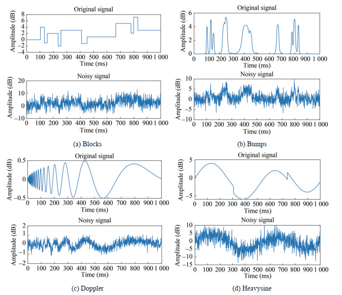Figure  3  Time-domain waveform of the noisy signal with 0 dB

Download: Full-Size Img

Taking the Heavysine signal as an example, Figure 3 shows the complete submersion of the Heavysine signal in noise. The following is the complete denoising process.

4.1   Signal decomposition

The noisy Heavysine signal is decomposed via EMD and EEMD methods (Figure 4). In both decomposition methods, the IMF1 represents the shortest oscillation period, typically corresponding to a noise component or high-frequency components.

Figure  4  Decomposition results of the noisy Heavysine signal with 0 dB

Download: Full-Size Img

4.2   Identifying noise and signal IMFs

The CC between each IMF component obtained through EMD and EEMD methods and the original signal is calculated (Figure 5).

Figure  5  CC curve of the noisy Heavysine signal obtained via EMD and EEMD

Download: Full-Size Img

Figure 5 reveals that the maximum curvature of CC curves occurs at the fourth-order position in EEMD and the sixth-order position in EMD. The first four IMFs can be classified as noise IMFs in EEMD, and the first six IMFs can be identified as noise IMFs in EMD.

4.3   Identifying noise-dominant IMFs

Noise-dominant IMFs can be identified based on the PEs of noise IMFs in EEMD. For the noisy Heavysine signal with an SNR of 0 dB, the PEs of noise IMFs are shown in Table 1. The PE of IMF4 is less than 0.75, indicating that IMF4 is the noise-dominant IMF in EEMD.

4.4   Denoising and reconstruction of noise-dominant IMFs

WSTD is applied to IMF4 using the wavelet basis function of db4 and a decomposition level of 4. The denoised Heavysine signal is obtained through the reconstruction of the denoised IMF4 and real IMFs. Figure 6 displays the denoising results. The denoising method that involves the use of wavelet soft-threshold method to directly eliminate signals is referred to as WSTD. Denoising methods that combine CC with EMD and EEMD are denoted as EMD–CC and EEMD–CC. The proposed denoising method is denoted as EEMD–CC–PE–WSTD.

Figure  6  Denoising results of the noisy Heavysine signal

Download: Full-Size Img

Figure 6 indicates that the denoised signal obtained through EEMD–CC–PE–WSTD can effectively fit the source signal. Sharp spikes are effectively eliminated, leading to a smoother and cleaner signal with minimal distortion. Compared with the signal obtained through the other three methods, the denoised signal obtained through the proposed method retains more features of the original signal. Moreover, the baseline of the denoised signal closely corresponds to that of the source signal, indicating effective baseline correction.

To further verify the effectiveness of the proposed method, four types of signals with different SNR_in are denoised through EMD–CC, EEMD–CC, WSTD, and EEMD–CC–PE–WSTD methods. Figures 7 and 8 show the denoising results.

Figure  7  SNR_out of different methods for simulated signals

Download: Full-Size Img

Figure  8  RMSE_out of different methods for simulated signals

Download: Full-Size Img

On average, EEMD–CC–PE–WSTD achieves the highest denoising effect. Particularly, at a low SNR_in, EEMD–CC–PE–WSTD features a significantly improved denoising performance. Additionally, EEMD–CC–PE–WSTD exhibits a higher SNR and lower RMSE than the other three denoising methods.

5   Denoising of measured ship signals

EMD–CC, EEMD–CC, WSTD, and EEMD–CC–PE–WSTD algorithms are used to denoise the ship sound signal from an open-source database to further verify the effectiveness of the proposed underwater acoustic denoising algorithm. Subsequently, SNR, RMSE, and CC are used to evaluate the denoising results.

5.1   Ship signal source

The ocean acoustic recordings used to train the classifier were obtained from various open-source databases. Ship noise data were collected from the ShipsEar (Santos-Domínguez et al., 2016). Most of these recordings were collected in or near the Port of Vigo using a hydrophone with a sampling rate of 52 734 Hz. Recordings from different types of vessels in or near the docks included fishing boats, ocean liners, ferries of various sizes, containers, tugs, pilot boats, yachts, and small sailboats. In this study, the audio recordings of passenger ships were selected for analysis to assess the performance of the denoising algorithm.

5.2   Signal preprocessing

To facilitate the subsequent denoising processing, we use a 0.6-s frame to crop the filtered target audio signal. To ensure the integrity of the signal during trimming, the overlapping duration between two adjacent frames of signals is set to 0.05 s. The signal-trimming process is shown in Figure 9.

Figure  9  Ship signal clipping process

Download: Full-Size Img

The time-domain diagram of the processed ship signal is shown in Figure 10.

Figure  10  Tested ship signal waveform

Download: Full-Size Img

The time-domain diagram of the collected ship signal contains numerous peaks and a significant amount of noise, indicating the need for denoising (Figure 10).

5.3   Selection of EEMD parameters for the ship signal

Notably, the A of the added white noise and the number of trials M are the two key parameters in EEMD. To select suitable parameters, the SNR of the ship signal after EEMD processing is calculated by varying A and M (Table 2).

Under a constant number of trials, a noise amplitude of 0.3 mV results in a maximum SNR value, while SNR decreases with increasing noise amplitude (Table 2). This is due to the effect of the added white noise on the signal, which increases overall noise and affects the decomposition results. At a constant noise amplitude of 0.3 mV, the maximum SNR value is achieved when M = 100. As the number of trials increases, the corresponding SNR value gradually stabilizes, indicating that excessively increasing the number of trials displays minimal effects on the decomposition results.

In summary, the experiment indicates that the optimal values are A = 0.3 mV and M = 100.

5.4   Ship signal denoising method

5.4.1   EMD–CC method

The processing effect of the decomposition of the ship signals obtained via EMD is shown in Figure 11. The ship signal decomposes into eight natural modal components through EMD (Figure 11). The first three components exhibit significant noise interference and mode mixing in the spectrogram. Subsequently, the signal is reconstructed, and the CC between each component and the original ship signal is calculated (Figure 12).

Figure  11  EMD decomposition components and spectrum diagram of ship signals

Download: Full-Size Img

Figure  12  EMD–CC variation curve of ship signal

Download: Full-Size Img

Figure 12 shows that the maximum curvature of CC occurs at the third-order position. The first three eigenmode components are considered noise signals and will be discarded, while the remaining components are classified as effective signals for reconstruction.

5.4.2   EEMD–CC method

The ship signal is decomposed using the two EEMD parameters determined in Figure 13.

Figure  13  EEMD decomposition components and spectrum diagram of ship signals

Download: Full-Size Img

EEMD decomposes the ship signal into six IMF components and sequentially separates the original ship signal from high-to-low frequency. Each component, starting from IMF2, exhibits a single signal scale, indicating the effective suppression of the modal mixing phenomenon. Additionally, the CC between each component and the original ship signal is calculated, and the results are shown in Figure 14.

Figure  14  EEMD–CC variation curve of ship signals

Download: Full-Size Img

Figure 14 reveals the point of maximum curvature in the CC curve corresponds to the third-order position. The first three IMF components are considered noise signals and will be discarded, and the remaining components are classified as valid signals for the reconstruction process.

5.4.3   EEMD–CC–PE–WSTD method

From section 5.4.2, the first three IMF components are identified as noise components, and the PE value of each component is calculated, as shown in Table 3.

The results revealed that the PE of IMF2 is less than 0.75. Thus, IMF2 can be considered the noise-dominant component and is denoised via WSTD. Additionally, the second IMF component is reconstructed along with the last three IMF components.

5.5   Comparison of different denoising results

Through the adjustment of the time axis, the time-domain diagram of the original signal is shown in Figure 15.

Figure  15  Time-domain diagrams of original ship signals

Download: Full-Size Img

The time-domain diagrams of the signal obtained from different denoising methods are shown in Figure 16.

Figure  16  Time-domain diagrams of the ship signal denoised via different methods

Download: Full-Size Img

All four methods effectively reduce peaks and glitches in the signal via denoising (Figure 16). However, the signal denoised via the proposed method is smoother and retains more valuable information compared with other methods. Additionally, the proposed method significantly reduces the impurities and noise in the signal, making it more favorable for human hearing.

Furthermore, the short-time Fourier transform diagram of the original signal is shown in Figure 17.

Figure  17  Short-time Fourier transform diagram of the original signal

Download: Full-Size Img

The short-time Fourier transform diagrams of the signal obtained via different denoising methods are shown in Figure 18.

Figure  18  Short-time Fourier transform diagram of the ship signal denoised via different methods

Download: Full-Size Img

For ship noise, the signal frequency range is mainly concentrated below 1000 Hz (Zhang et al., 2017). Figures 17 and 18 show the wide frequency distribution of the original signal, particularly with various frequency components present above 1 000 Hz. However, the frequency of the denoised signal is highly concentrated, mainly below 5 000 Hz, and the background noise is significantly reduced. Furthermore, the algorithm proposed in this paper exhibits a more significant denoising effect on the signal, with the signal mainly concentrated below 1 000 Hz.

5.6   Denoising effect evaluation

The following three parameters are used to evaluate the denoising effect of actual underwater acoustic signals (Table 4).

Table 4 indicates that the SNR of the reconstructed signal is improved using WSTD, EMD, and EEMD algorithms. Moreover, the SNR of the signal reconstructed through the improved EEMD method is 14 dB higher than that of the original signal. The RMSE and CC results revealed that signals processed through the improved EEMD exhibit lower RMSE and higher CC than the original signal. Therefore, the EEMD–CC–PE–WSTD algorithm exhibits an improved denoising effect and is effective and suitable for denoising underwater acoustic signals.

6   Conclusions

To reduce the loss of effective signals during the denoising process of underwater acoustic signals, a noise reduction method based on EEMD, which incorporates CC, PE, and WSTD is proposed. The key innovations and conclusions of the proposed denoising method are as follows:

1) The adaptive decomposition algorithm, EEMD, is used to denoise underwater acoustic data signal. This process decomposes original data into a set of IMF components with different scales.

2) Compared with existing denoising methods, CC and PE classify IMFs into three parts (pure noise IMFs, noise-dominant IMFs, and real IMFs).

3) The curvature value of the CC curve is used to distinguish between the noise and real components of the underwater acoustic signal based on the characteristics of the signal without the need for an arbitrary threshold.

4) The proposed EEMD–CC–PE–WSTD method does not require human intervention. The calculation process is adaptive.

5) Four types of signals (Blocks, Bumps, Doppler, and Heavysine) with different SNRs are denoised through EMD–CC, EEMD–CC, EEMD–CC–PE–WSTD, and WSTD methods. The proposed denoising method exhibits higher performance, with lower RMSE and higher SNR.

6) Compared with other denoising methods, the EEMD–CC–PE–WSTD method is an effective method for denoising underwater acoustic signals. This study provides a solid foundation for the subsequent processing of ship-radiated noise signals, including prediction, detection, extraction, and classification.