1   Introduction

Hydrofoil, as a typical lifting body, is widely used in the fields of ships and hydraulic machinery. Marine rudders, fin stabilizers, planing wings of hydrofoils, various control surfaces of underwater vehicles, and blades of propellers and hydraulic turbines are all hydrofoil structures. The use of hydrofoil technology also provides greater maneuvering stability, particularly with respect to changes in wave elevation (Mahmud, 2015). Because a hydrofoil is an elastic body, it can vibrate and deform under the action of fluid loads. Due to the complex and variable flow field environment in which it works, its vibration response can also change significantly, with strong unsteady characteristics. If the design of hydrofoils is not reasonable, the fluid may stimulate hydrofoils to flutter as the speed increases, threatening the safety of the structure. Flutter is a self-excited vibration phenomenon, in which the fluid excites the hydrofoil structure to vibrate, and the vibration in turn can disturb the flow field and change the distribution characteristics of the load. If the changing fluid load happens to have a negative damping effect on the hydrofoil, the fluid will not contribute to structural stability. At this time, the system will continue to obtain energy from the fluid, and instability with gradually expanding amplitude will occur, ultimately causing structural damage and failure, which is a dangerous situation that needs to be avoided. Uncontrolled static and/or dynamic instabilities can lead to excessive deformation, material failure, accelerated fatigue, vibration, noise issues, and even catastrophic structural failures (Abramson, 1969; A. Kousen and O. Bendiksen, 1988; O. Bendiksen, 1992; Bendiksen, 2002).

The early research on flow-induced vibration of airfoil structures was mainly focused on the field of aviation engineering, which was used to guide the aeroelastic design of aircraft and solve wing flutter problems. Researchers mainly used linear potential flow theory to analyze and study the aerodynamic characteristics of two-dimensional elastic wings, and had obtained some important theoretical results, especially the unsteady aerodynamic theory proposed by Theodorsen (Theodorsen, 1935; Theodorsen and Garrick, 1940), which laid the foundation for the aeroelastic stability and flutter analysis of airfoil structures. Lottati et al. (Lottati, 1985; Smith and Chopra, 1990; Wu and Sun, 1991; White and Heppler, 1995; Banerjee, 2001) solved the flutter characteristics of box beams, Timoshenko beams (vertically and horizontally curved beams), and thin-walled beams using spline methods based on Theodorsen's aeroelastic theory and wing theory, verifying the wide applicability of this method. Zhang (Zhang et al., 2019) proposed a low-cost and low-risk flutter boundary prediction method, which requires only one upwind test at subcritical velocity. Even if the reference dynamic pressure is far from the flutter critical point, it can also have a certain prediction accuracy for flutter occurrence. Jonsson (Jonsson et al., 2019) reviewed the methods of flutter analysis in aircraft design optimization and summarized the research status and main problems in this field. In the field of hydrodynamics, with the gradual development of ships towards high speed and large scale, the hydrodynamic loads borne by structures continue to increase, placing higher requirements for structural safety and reliability. The vibration and hydroelasticity of underwater structures have also become noticeable, especially for various prominent hydrofoil appendages. Therefore, in recent years, more and more research has been conducted on the flow-induced vibration of hydrofoils. Currently, the main methods include experimental testing and numerical calculation.

In terms of experiments, the following scholars have conducted relevant research work. Taking the rudder shaft system as the research object, Jewell (Jewell and McCormick, 1961) had demonstrated through a large number of experiments that the Theodorsen 2-DOF motion equation, which is widely used in aerodynamics, is also applicable to underwater lifting bodies. Ducoin (Ducoin et al., 2012) conducted a water tunnel test on the structural response of a cantilever flexible hydrofoil with or without cavitation, and measured the displacement deformation and surface vibration velocity of the free end of the hydrofoil using a high-speed camera and a laser doppler vibrometer. The research showed that the response of the hydrofoil under non-cavitation flow is closely related to the hydrodynamic load affected by viscosity, and the unsteady hydrodynamic force caused by cavitation can significantly increase the vibration level. At the same time, it will cause the attached water mass to decrease and affect the response frequency of some modes of the structure. Harwood (Harwood et al., 2019a; 2019b) conducted experiments on a rigid variant and two flexible variants of a vertical surface-piercing hydrofoil in wetted, ventilating and cavitating conditions, describing the dynamic FSI response of a flexible surface-piercing hydrofoil in dry, wetted, ventilating and cavitating conditions. Smith (Smith et al., 2020a; 2020b, Young et al., 2022) used high-speed camera and synchronous force measurements to study the effects of fluid-structure interaction on rigid and flexible hydrofoil cloud cavitation in a variable pressure water tunnel and explained the complex response. Herath (Herath et al., 2021) conducted cavitation tunnel tests on optimized shape adaptive composite hydrofoils and compared the results with other composite hydrofoils. The study found that hydrofoils can have significantly different responses for the same Reynolds number if the flow velocity is different. Liu (Liu et al., 2021; 2023) used a synchronous measurement system consisting of a high-speed camera, a hydrodynamic load cell, and a Laser Doppler Vibrometer to study the dynamics of sheet/cloud cavitation in fluid-structure interaction, and summarized the effects of bend-twist coupling on the cavitation behavior and hydroelastic response of composite hydrofoils.

Compared to experimental testing, using numerical methods to predict the hydroelastic response of hydrofoils can save manpower and material resources, and obtain more flow field and vibration information, which is helpful to reveal the flow-induced vibration laws of hydrofoils. With the emergence of workstations and large-scale computers, fluid-structure interaction numerical methods combining computational fluid dynamics (CFD) and computational structural dynamics (CSD) have become an effective means to solve vibration problems of underwater structures. Kinnas (Kinnas and Fine, 1993, Senocak and Wei, 2002) conducted a large number of numerical studies on the cavitation response of rigid hydrofoils, but their research on flexible hydrofoils was limited. Ducoin (Ducoin et al., 2010) solved the fluid-structure interaction problem of a hydrofoil with 2-DOF, bending and twisting, based on the commercial computational fluid dynamics software STAR-CCM+. The results showed that the motion of the hydrofoil increases the angle of attack, leading to an increase in lift and drag coefficients and an increase in cavitation length. Chae (Chae et al., 2013) coupled the unsteady RANS solver with a two-degrees-of-freedom (2-DOF) structural model to explore the effects of relative mass ratio and viscous effects on the fluid-structure interaction response and stability of hydrofoils. The results showed that the instability modes of hydrofoils are divergent, dynamic divergent, and flutter in different relative mass ratio regions. Ducoin (Ducoin and Young, 2013) simplified the flexible hydrofoil into a 2-DOF system and calculated the static divergence velocity using CFX. The results showed that the viscous effect moves the pressure center toward the middle of the hydrofoil at large angles of attack, which helps to delay or suppress divergence. Wang (Wang et al., 2009) examined the effect of different locations of the pitching axis on propulsive performance of a two-dimensional flexible fin, the results showed that maximum thrust can be achieved with the pitching axis at the trailing edge. The static fluid-structure interaction simulation results of Huang (Huang et al., 2019) showed that compared to unidirectional fluid-structure interaction, the flexible hydrofoil has a lower lift and greater resistance when subjected to bidirectional fluid-structure interaction. Liu (Liu et al., 2019) used dynamic mode decomposition (DMD) and inherent orthogonal decomposition (POD) to analyze the coherent structure of cavitation flow over ALE-15 hydrofoils. The results showed that DMD is more effective in decomposing complex flow fields into uncoupled coherent structures with specific dynamic modes and corresponding frequencies than POD. Xu (Xu and Tang, 2020) simulated the flow field of a NACA66-mod hydrofoil under different trailing edge vibration amplitudes and frequencies, and the results showed that the vibration amplitudes and frequencies have a significant impact on trailing edge vortex shedding. Chae (Chae and Young, 2021) discussed the effects of key geometric parameters, material parameters, and flow parameters on the steady-state and dynamic responses of spanwise flexible airfoils and hydrofoils. The results showed that the main instability of hydrofoils is divergence, while the main instability of airfoils is flutter. Hou (Hou et al., 2013) studied the effects of geometric parameters of the rudder on the hydrodynamic performance of the propeller-rudder system, the calculation results showed that the rudder span has an optimal match range with the propeller diameter. George (George and Ducoin, 2021) used the direct numerical simulation (DNS) method to simulate three-dimensional incompressible flow, and the results showed that vibration has a significant impact on the pressure gradient of hydrofoils, thereby changing the transition position and boundary layer characteristics that are proportional to the vibration amplitude and frequency ratio. Negi (Negi et al., 2021) conducted a global linear stability analysis of the fluid-structure interaction problem of NACA0012 airfoil at transition Reynolds numbers and studied the spontaneous pitch oscillation phenomenon. The results showed that the aeroelastic instability is caused by the linear instability mode of the fluid-structure interaction problem. Wang (Wang et al., 2021) presented a multi-scale Eulerian-Lagrangian approach to simulate cavitating turbulent flow around a Clark-Y hydrofoil to study the bubble dynamics. The results showed that the pressure wave released as a bubble is compressed reaches 10⁷ Pa, which may cause cavitation erosion of the hydrofoil surface.

Due to the tremendous damage that the flutter can cause to structures, many studies have been conducted on the flow-induced vibration of hydrofoils. However, most of the current research focuses on the flow-induced vibration characteristics of flexible hydrofoils or the cavitation response of rigid hydrofoils, while there are few studies on the flow-induced vibration characteristics of rigid hydrofoils. At the same time, theoretical formulas are often used to derive the flutter critical velocity, and corresponding numerical studies are lacking. In response to these two shortcomings, the research goal of this article is to study the flow-induced vibration characteristics of a rigid hydrofoil with 2-DOF under uniform flow through numerical simulation, in order to avoid the occurrence of flutter. This work complements previous research and has a certain reference value. Firstly, the flow field model and structural model of this numerical simulation are introduced; Then, the dynamic responses under different velocities and angles of attack are analyzed, and the effects of natural frequency ratio and inertia radius on the vibration state of hydrofoils are compared; Finally, the work of this article is summarized, and the shortcomings and directions for further research are pointed out.

2   Numerical model

Based on the co-simulation of computational fluid dynamics (CFD) and structural finite element method (FEM), this work performs a bidirectional fluid-structure interaction calculation and conducts a numerical simulation study on the flow-induced vibration of a three-dimensional elastic hydrofoil to obtain the dynamic response characteristics of the hydrofoil at different velocities and angles of attack. At each time step, the three-dimensional hydrodynamic load is calculated by the CFD numerical model, and the pressure and shear force are imported into the FEM through the fluid-structure interface to solve the structural response. The three-dimensional structural displacement is then imported into the flow field to achieve the update of the flow field grid, and the hydrodynamic load and structural response are recalculated. The calculation repeats the iteration until the solution variable converges or the maximum internal iteration number is reached, and then the next time step is started. The fluid-structure coupling calculation process is shown in Figure 1.

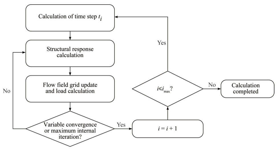Figure  1  The fluid-structure coupling calculation process

Download: Full-Size Img

Section 2.1 verifies the effectiveness of this calculation method using the NACA66 flexible hydrofoils. Subsequently, this method is further applied to calculate 2-DOF NACA66 rigid hydrofoils. Sections 2.2 and 2.3 respectively describe the flow field model and structural model of the 2-DOF NACA66 rigid hydrofoil used in this work.

2.1   Numerical model validation

Ducoin conducted flow-induced tests on NACA66 flexible hydrofoils at different cavitation numbers in a water tunnel (Ducoin et al., 2012). This section verifies the effectiveness of the fluid-structure interaction method concerning non-cavitation conditions. The chord length of hydrofoil is 0.148 m, and the extension length is 0.191 m. One end is fixed to the wall of the water tunnel, and the other end is free. The cross-sectional dimension of the water tunnel is 0.192 m×0.192 m. Based on Star-CCM+ and Abaqus, a bidirectional fluid-structure interaction calculation was conducted for the NACA66 hydrofoil. The fluid calculation domain was 1 m long, with a velocity inlet at the left end, a pressure outlet at the right end, and a non-slip wall around. Large eddy simulation was used for calculation. The mesh is divided using a cutting volume method. The dimensionless thickness of the first layer of mesh near the wall meets y⁺<1, and the total number of meshes is 3.25 million. The flow field mesh scene is shown in Figure 2.

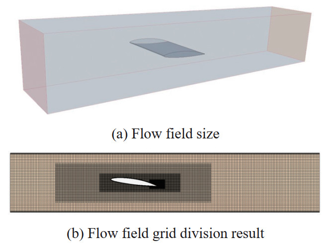Figure  2  Flow field grid

Download: Full-Size Img

The hydrofoil material is polyoxymethylene, with a density of ρ=1 480 kg/m³, Young's modulus of E=3.0 GPa, and a Poisson's ratio of ϑ=0.35. The mesh is discretized using a second-order hexahedral element C3D20R. The finite element model is shown in Figure 3. The natural frequency and modal calculation results of the hydrofoil are shown in Table 1 and Figure 4. It can be seen that the vibration modes of the hydrofoil in vacuum and in water are basically the same, with the first three vibration modes being first-order bending, first-order pitch, and second-order bending. However, due to the high density of water, the natural frequencies in water are significantly lower than those in real air. Comparing the wet mode natural frequencies with the results given by Ducoin, it can be seen that the two modes are basically consistent.

Figure  3  NACA66 flexible hydrofoil finite element model

Download: Full-Size Img

Figure  4  First three modal shapes

Download: Full-Size Img

After that, a fluid-structure interaction calculation was performed, with an incoming flow velocity of 5 m/s, and the structure was solved using implicit dynamic solutions. The vertical displacement of the monitoring point at the free end guide edge of the hydrofoil at 4°, 6°, and 8° angles of attack is shown in Figure 5. It can be seen that the vibration gradually attenuates and eventually fluctuates slightly around a constant value. The larger the angle of attack, the higher the equilibrium position. The mean value of the stable section is in good agreement with the experimental values given in the literature (Ducoin and Young, 2013), which verifies the effectiveness of the fluid-structure coupling calculation method in this work.

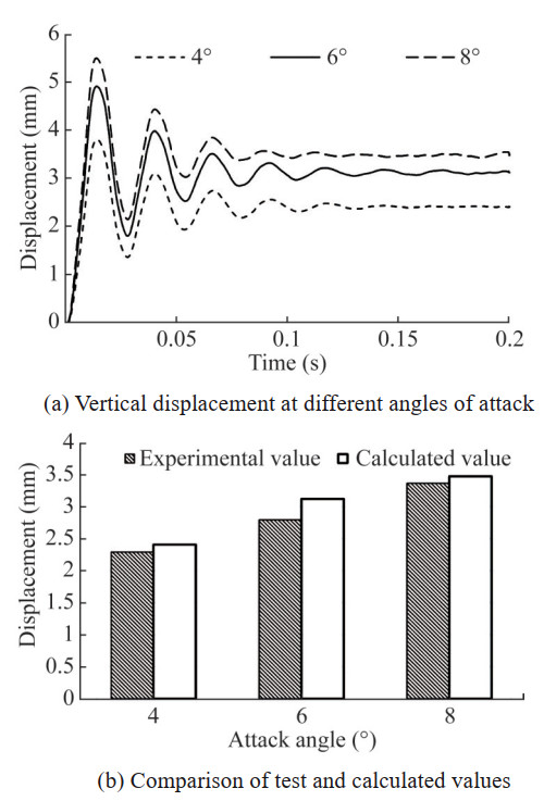Figure  5  Comparison between calculated displacement value and test value

Download: Full-Size Img

Based on the aforementioned calculation method, this work also compared the lift coefficients with the experimental data. The experimental data were obtained from testing a hydrofoil with the NACA66 series, having a chord length of 0.150 m and a span of 0.191 m, at a nominal freestream velocity of 5.33 m/s and at 4°, 6°, and 8° angles of attack. The measured and predicted lift and drag coefficients of the hydrofoil at these angles are given in Table 2. The numerical results are consistent with the experimental data given in the literature (Leroux et al., 2004), which verifies the effectiveness of the numerical model in this work.

2.2   Flow field model

The hydrofoil has a section shape of NACA66 airfoil with a chord length of c=0.148 m. The fluid density is 997.561 kg/m³ and the kinematic viscosity coefficient is 1.012 5 mm²/s. The upstream and upper/lower boundaries of the flow field are set as velocity inlets, and the downstream boundary is set as a pressure outlet. The ratio of the spanwise width of the flow field to the chord length of the hydrofoil is 1∶3. Both sides are taken as symmetrical planes to reduce the number of grids in the flow field and structure and the computational cost of fluid-structure interaction. The grid is divided using a cutting volume method and locally densified. The mesh near the wall meets the requirements of y⁺<1. Change the basic size of the grid to divide three sets of flow field grids, with grid amounts of 2.08 million, 3.17 million, and 7 million, respectively. The 3.17 million grid case is shown in Figure 6. The grid independence verification of the flow field is performed at a 6° angle of attack and a 5 m/s flow velocity. The time step is 4×10⁻⁴ s. The SST k−ω DES turbulence model is used for calculation, and the average value of the hydrofoil lift coefficient is monitored. The results are shown in Table 3. The difference percentage of the lift coefficient is defined as (Cl − Cl_m)/Cl_m, where Cl_m is the lift coefficient of the maximum grid quantity model. It can be seen that the lift coefficient basically converges when the grid quantity is 3.17 million and 7 million.

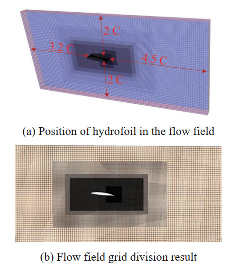Figure  6  2-DOF hydrofoil flow field grid

Download: Full-Size Img

Based on a comparison of the calculation results of three time steps 2×10⁻⁴ s, 4×10⁻⁴ s, and 8×10⁻⁴ s based on a 3.17 million grid, as shown in Table 4, it can be seen that the lift coefficient difference is small when the time steps are 2×10⁻⁴ s and 4×10⁻⁴ s. Considering the calculation accuracy and time length, a 3.17 million grid combined with a time step of 4×10⁻⁴ s is selected for subsequent calculation.

2.3   Structural model

As shown in Section 2.1, the numerical model is validated based on three-dimensional flow. In the following investigations, the flow fields are also chosen to be three dimensional. It is worth pointing out that the simulated hydrofoil has the same NACA66 cross section, however, it is rigid body and moves with heave and pitch motions only, as shown in Figure 7. It is simulated to represent a section of the 3-DOF hydrofoil in order to focus on the interaction between the hydrofoil vibration and the vortex shedding without the distraction of the three-dimensional deformation, as well as reduce the computational costs of multiple simulations.

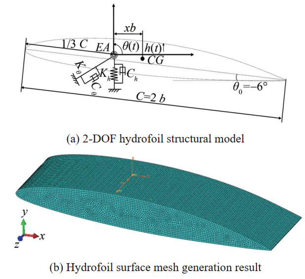Figure  7  2-DOF rigid hydrofoil

Download: Full-Size Img

The elastic axis is located at one third of the chord length from the leading edge, and a center of gravity CG located at the geometric center between the elastic axis and the trailing edge. x is the horizontal dimensionless distance from the elastic axis, S and I are the static moment and moment of inertia of the hydrofoil about the elastic axis. The natural frequencies of pure heave and pure pitch motions of hydrofoils are the same, both are 9.5 Hz. The calculation formula for relevant parameters is as follows:

The relevant operating data and the geometrical of the hydrofoil are shown in Table 5.

The vibration equation for a 3-dimensional rigid wing with 2-DOF can be expressed as:

where M_S, C_S, and K_S are, respectively, the structural inertial, damping, and stiffness matrices, while X, $\dot{\boldsymbol{X}} $, and $\ddot{\boldsymbol{X}}$ are, respectively, the structural displacement, velocity, and acceleration vectors with X = [ h, θ ]^T. Furthermore, F = [ L, M ]^T is the fluid force vector.

where m, S_θ, and I_θ are, respectively, the structural mass, the static imbalance, and the structural moment of inertia defined about the E.A., while C_h and C_θ, K_h and K_θ are, respectively, the structural damping values for the bending and twisting motions, the structural bending and torsional stiffness values. The overhead dots indicate Lagrangian time derivatives and hence h, $\dot{h}$, and $\ddot{h}$ are, respectively, the bending displacement, velocity, and acceleration, while θ, $\dot{\theta}$, and $\ddot{\theta}$ are, respectively, the twisting displacement, velocity, and acceleration. L and M are the fluid lift and moment acting on the foil, defining the heave motion as positive upward and the pitch motion as positive counterclockwise.

The expression of L_h, L_θ, M_h, M_θ in the formula are: If the right side of the equation is 0, and the hydrofoil parameters are substituted into the equation, the natural frequencies of the 2-DOF undamped system can be obtained to be 7.77 Hz and 12.95 Hz, respectively.

When hydrofoil flutter occurs under fluid excitation, its vibration state approximates simple harmonic motion. Theodorsen has derived the unsteady forces and moments on two-dimensional thin wings that vibrate harmonically at the angular frequency ω in incompressible uniform flow. Based on this theory, the flutter critical velocities of 2-DOF hydrofoils are predicted. The derivation of the unsteady forces and moments is relatively complex. Here, the expressions for the unsteady lift L and moment M of a hydrofoil with a span of l are directly given:

where ρ is the density of the medium, V is the inflow velocity, a is the dimensionless distance of the hydrofoil mid-point from the elastic axis, backward is positive, the reduction frequency k, and C(k) is the Theodorsen function.

where J₀, J₁, Y₀, Y₁ is the first and second type of standard Bessel functions of k, respectively.

Substituting Eq. (7) into (4) and (5) can obtain:

Substituting Eqs. (7), (8) and (9) into the vibration Eq. (3) of a 2-DOF hydrofoil can obtain:

To make the equations solvable, the determinant of the left coefficient matrix is 0. However, the coefficient matrix contains two unknown variables, the reduced frequency k and the vibration angular frequency ω. k exists in the coefficient L_h, L_θ, M_h, M_θ and cannot be directly solved. Here, the V-g method is used to solve the flutter determinant. Artificial damping is introduced into the vibration Eq. (3), so that the damping forces on the 2-DOF are −igk_hh and −igk_θθ, respectively. At this time, the flutter determinant becomes:

By substituting $Z=(1+i g)\left(\frac{\omega_\theta}{\omega}\right)^2$ into the above equation, we can obtain a one-dimensional quadratic equation about Z. However, it is necessary to know the value of the coefficient L_h, L_θ, M_h, M_θ to solve the root of the equation.

Here, we can assume a series of k values, for each k, we can obtain a set of L_h, L_θ, M_h, M_θ values, and solve the two complex roots $Z=Z_R+i Z_I$ about Z. At the same time, we can determine the vibration angular frequency ω, artificial damping g, and inflow velocity V based on the following relationships:

Plot each set of V and g values obtained, with the horizontal axis being V and the vertical axis being g. When g<0, it is necessary to provide negative damping to maintain simple harmonic vibration of the hydrofoil, that is, to input energy to the system, indicating that flutter will not occur in the hydrofoil vibration at this flow velocity; When g>0, it is necessary to provide damping to consume system energy to generate simple harmonic vibration, indicating that flutter has occurred on the hydrofoil at this flow velocity; When g=0, the hydrofoil can maintain simple harmonic vibration only under fluid excitation, and the corresponding V is the critical velocity of flutter.

Next, the parameters of the hydrofoil structural model are substituted into the flutter Eq. (12) and calculated using the V-g method. Given a series of k values, the corresponding V-g curve is obtained, as shown in Figure 8. It can be seen that as the inflow velocity increases, the value of g changes from a negative value to a positive value, and the trend of change decreases first and then increases. When g=0, the corresponding inflow velocity V=4.5 m/s, so the flutter critical velocity calculated by the V-g method is 4.5 m/s.

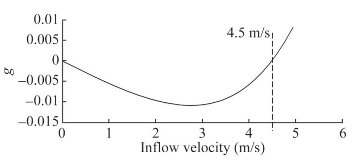Figure  8  V-g figure

Download: Full-Size Img

3   Results and discussion

This chapter focuses on analyzing the heave displacement, pitch angle, hydrodynamic force, and real-time energy exchange between fluid and elastic systems, analyzing the dynamic response under different flow velocities and angles of attack, and comparing the effects of hydrofoil natural frequency ratios and inertial radius on vibration states.

3.1   Dynamic response of hydrofoil at different velocities

This section presents the dynamic response of a 2-DOF hydrofoil at velocities V=1 m/s, 3 m/s, 4.5 m/s, 5 m/s, and 6 m/s, with an initial angle of attack of 6°. When V=1 m/s, the curves of heave displacement, pitch angle, lift, and the torque of the fluid to the elastic axis are shown in Figure 9. It can be seen that the amplitude of heave and pitch motion attenuates with time. The spectrum results in Figure 10 shows that heave and pitch vibration contain two main frequency components, 7.3 Hz and 12.2 Hz, respectively, which are close to the first-order and second-order natural frequencies of the undamped system. The vibration is greatly affected by the natural characteristics of the hydrofoil. The non-dimensional Froude number, vibration state, maximum power and average work for each velocity are shown in Table 6. The maximum power and average work are taken from the last cycle of the critical state, and the calculation formula for Froude number is as follows:

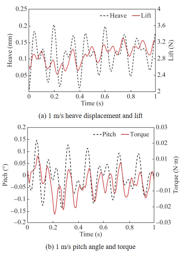Figure  9  Vibration and hydrodynamic force time history results (1 m/s)

Download: Full-Size Img

Figure  10  Heave and pitch motion spectrum results (1 m/s)

Download: Full-Size Img

where V is the inflow velocity, g value is 9.81 m/s², and c is the chord length of hydrofoil.

To observe the flow field and the energy exchange of a 2-DOF elastic system, calculate the hydrodynamic power P(t) and the total work W(t) it does to the system at different times. The results are shown in Figure 11. It can be seen that the amplitude of hydrodynamic power and the total work done to the elastic system have a downward trend, indicating that the intensity of energy exchange between the fluid and the hydrofoil has decreased, and the energy of the elastic system has a downward trend, at which time the vibration of the hydrofoil is in a convergent state.

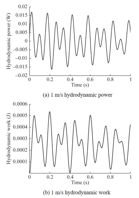Figure  11  Hydrodynamic power and work history results (1 m/s)

Download: Full-Size Img

where $\dot{h}$ and $\dot{\theta}$ are the heave velocities and pitch angular velocities, and the lift and fluid torque received by the elastic axis are L (t) and M (t).

The dynamic response of the hydrofoil at V=3 m/s is shown in Figures 12‒14. Compared to V=1 m/s, the amplitudes of heave and pitch motions significantly increase, but the attenuation trend decreases. In addition, there is only one main frequency component remaining in the vibration spectrum, 12.2 Hz, and the amplitudes of other frequency components are small. The vibration of the system starts to be dominated by a single frequency. At this point, the amplitude of the hydrodynamic power does not significantly attenuate, while the maximum amplitude of the total work of the fluid still decreases from 0.4 seconds, indicating that as the number of vibration cycles increases, the fluid will dissipate the energy of the system, and the vibration is still in a convergent state.

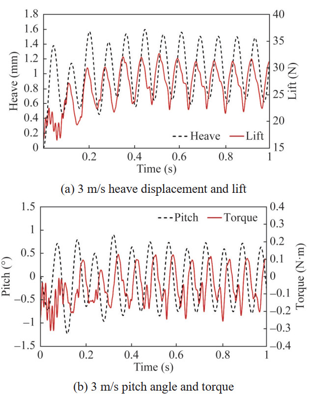Figure  12  Vibration and hydrodynamic force time history results (3 m/s)

Download: Full-Size Img

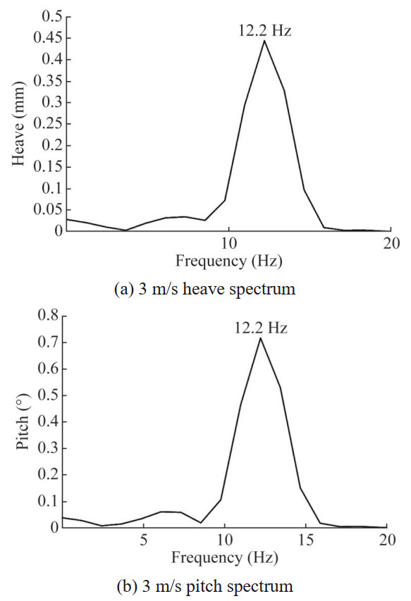Figure  13  Heave and pitch motion spectrum results (3 m/s)

Download: Full-Size Img

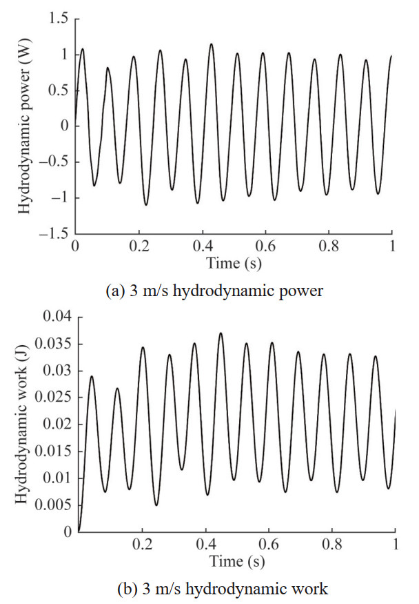Figure  14  Hydrodynamic power and work history results (3 m/s)

Download: Full-Size Img

The time history results of hydrofoil vibration and hydrodynamic work at V=4.5 m/s are shown in Figures 15 and 16. The amplitudes of heave displacement, pitch angle, and lift and torque decay rapidly over time. According to the average time interval of vibration peaks, the vibration frequencies of both degrees of freedom are 11.8 Hz. The negative work of hydrodynamic force in each vibration cycle is higher than the positive work, and the overall damping effect is negative. The system energy continuously decreases, and the vibration is in a convergent state.

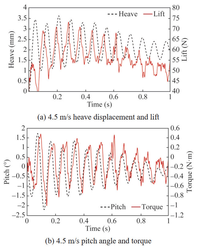Figure  15  Vibration and hydrodynamic force time history results (4.5 m/s)

Download: Full-Size Img

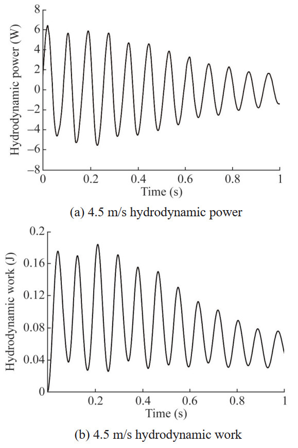Figure  16  Hydrodynamic power and work history results (4.5 m/s)

Download: Full-Size Img

When the inflow velocity V increases to 5 m/s, the dynamic response of the hydrofoil is shown in Figures 17‒19. It can be seen that the amplitudes of heave and pitch motions continue to increase without a trend of attenuation, and the vibrations of the 2-DOF are still dominated by a single frequency, both 11.6 Hz. At the same time, the amplitude of hydrodynamic power no longer attenuates, and the total work of the fluid presents a slightly increasing trend with the increase of the vibration period. The energy input to the system begins to accumulate, which determines that the 5 m/s flow velocity of the hydrofoil is in an unstable state, that is, a critical state of flutter. It can be seen that the flutter critical velocity of the numerical simulation is higher than the theoretical calculation value of 4.5 m/s based on the Theodorsen unsteady force in Section 2.3. This is mainly because the derivation of the Theodorsen unsteady force is based on the potential flow method, without considering viscosity and specific hydrofoil shape, and the expression is a solution in the frequency domain. Although the numerical simulation takes a long time to calculate, it can fully consider the hydrofoil shape, In the time domain, the unsteady force and hydrofoil response are directly solved based on the CFD method.

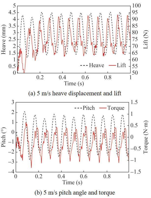Figure  17  Vibration and hydrodynamic force time history results (5 m/s)

Download: Full-Size Img

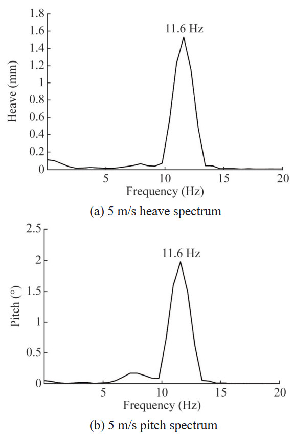Figure  18  Heave and pitch motion spectrum results (5 m/s)

Download: Full-Size Img

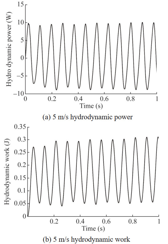Figure  19  Hydrodynamic power and work history results (5 m/s)

Download: Full-Size Img

Continue to increase the incoming flow velocity, and the results at V=6 m/s are shown in Figures 20‒22. At this point, the vibration of the hydrofoil enters a flutter state, and the amplitudes of the heave and pitch motions gradually increase with time. The frequency spectrum shows that both the heave and pitch frequencies are 11 Hz, which is somewhat lower than the critical state. This may be due to the rapid increase in the amplitude of the hydrofoil in the flutter state and the greater impact of the attached fluid. In addition, the power amplitude and total work of this hydrodynamic force also multiply with the increase of the vibration period, and the system continuously obtains energy from the fluid until damage occurs.

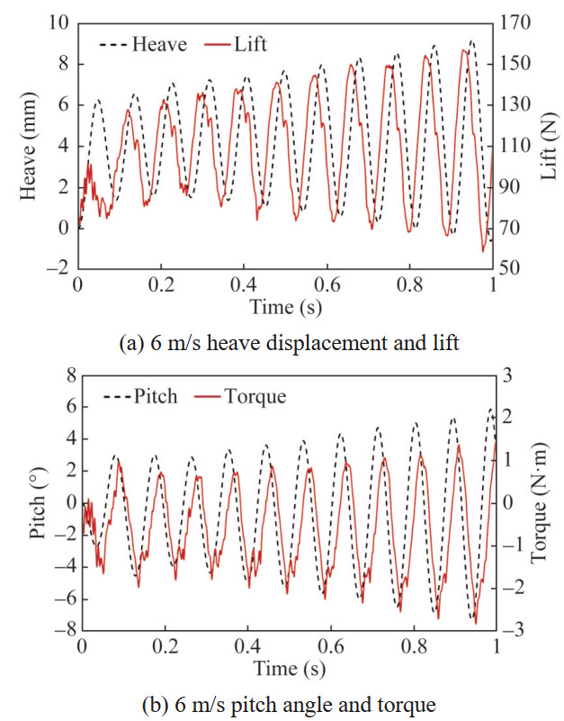Figure  20  Vibration and hydrodynamic force time history results (6 m/s)

Download: Full-Size Img

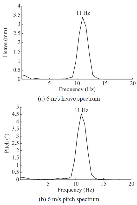Figure  21  Heave and pitch motion spectrum results (6 m/s)

Download: Full-Size Img

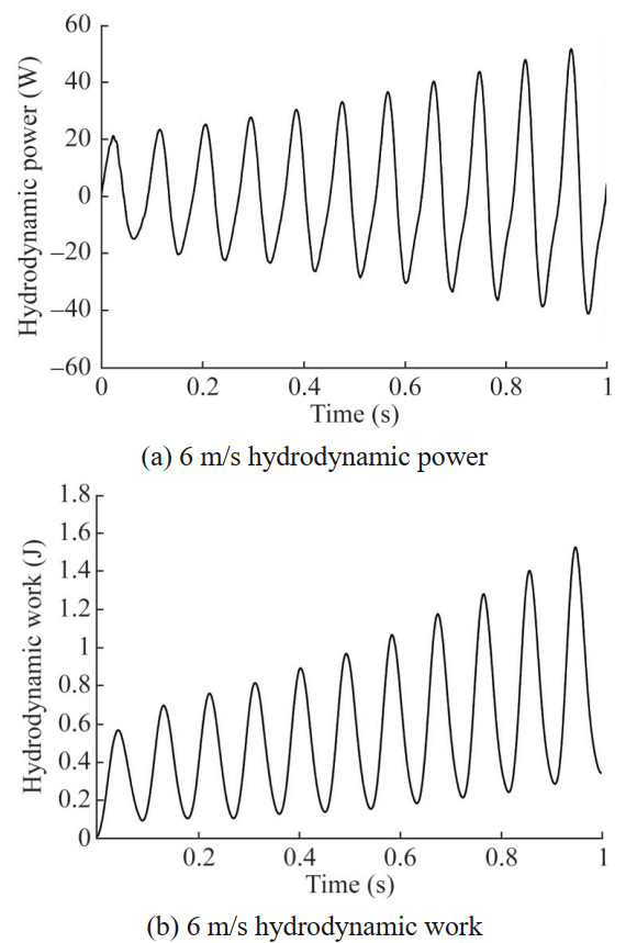Figure  22  Hydrodynamic power and work history results (6 m/s)

Download: Full-Size Img

The flow field vorticity results of the midspan cross section of the hydrofoil in the critical and flutter states are shown in Figure 23. Corresponding to the last complete cycle T in the hydrodynamic power curve, the hydrodynamic power is 0 at 0 and T, positive at T/5 and 2T/5, and negative at 3T/5 and 4T/5. The flow field vorticity results of the three-dimensional hydrofoil in the critical and flutter states at the final moment are shown in Figure 24. During the entire vibration cycle of the critical state, vortices are mainly generated in the middle and rear parts of the hydrofoil. With the constant change of the attack angle of the hydrofoil, they are brought into the wake flow field by the main stream to form relatively fine shedding vortices. In the case of flutter, the vorticity of the suction surface is still concentrated in the rear region during the upstroke of the hydrofoil. However, during the downstroke, a series of significant vortices are generated in the middle and front of the suction surface, which are then dispersed by the incoming flow and merged into the vortex at the rear as the angle of attack decreases. This is mainly due to the large response of the hydrofoil to the heaving and pitching motions during the flutter state, and the rapid replenishment of surrounding fluid to the suction side surface during the downstroke.

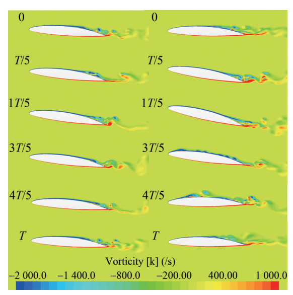Figure  23  Flow field vorticity results of the midspan cross section of the hydrofoil (left: critical state, right: flutter state)

Download: Full-Size Img

Figure  24  Flow field vorticity results of the three-dimensional hydrofoil

Download: Full-Size Img

3.2   Dynamic response of hydrofoil at different angles of attack

Other conditions remain unchanged, changing the initial angle of attack to 4° and 8°, and calculating the flow-induced response at a flow velocity of 5 m/s. The vibration state, maximum power and average work for each angle of attack are shown in Table 7. The vibration and hydrodynamic results at different angles of attack are shown in Figures 25 and 26.

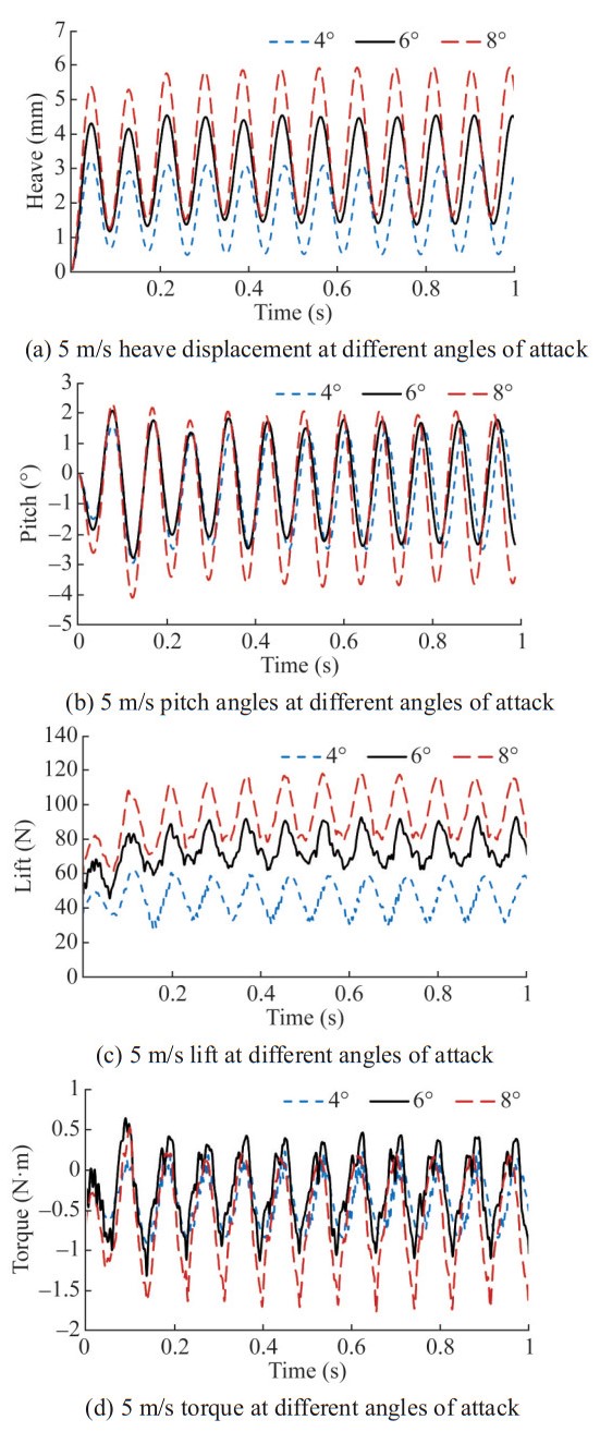Figure  25  Vibration and hydrodynamic force time history results at different angles of attack (5 m/s)

Download: Full-Size Img

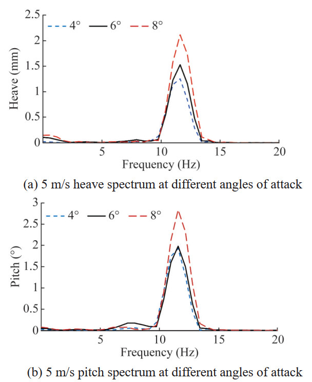Figure  26  Spectrum results of heave and pitch motions at different angles of attack (5 m/s)

Download: Full-Size Img

After adjusting the angle of attack to 4° and 8°, the heave and pitch vibrations of the hydrofoil do not attenuate or expand, but maintain constant amplitude vibration. As the angle of attack increases, the average lift increases, and the oscillation amplitude and equilibrium position of the heave motion also significantly increase. Compared to 4° angle of attack, the pitch amplitude increases slightly at 6° angle of attack, while it increases significantly at 8° angle of attack, consistent with the variation of torque. In addition, the peak frequencies of heave and pitch vibrations at 4°, 6°, and 8° attack angles are all around 11.6 Hz, indicating that changes in the initial attack angle have a small impact on the vibration frequency. Figure 27 shows the fluid work situation, and the results show that the oscillation amplitude of the hydrodynamic power and work curve increases significantly with the increase of the angle of attack, and there is no attenuation trend and gradually tends to stabilize. Based on the vibration curve, it can be judged that the hydrofoil at 4° and 8° angles of attack is still in a critical state, that is, a small change in the initial angle of attack has no significant impact on the critical flutter speed of the hydrofoil.

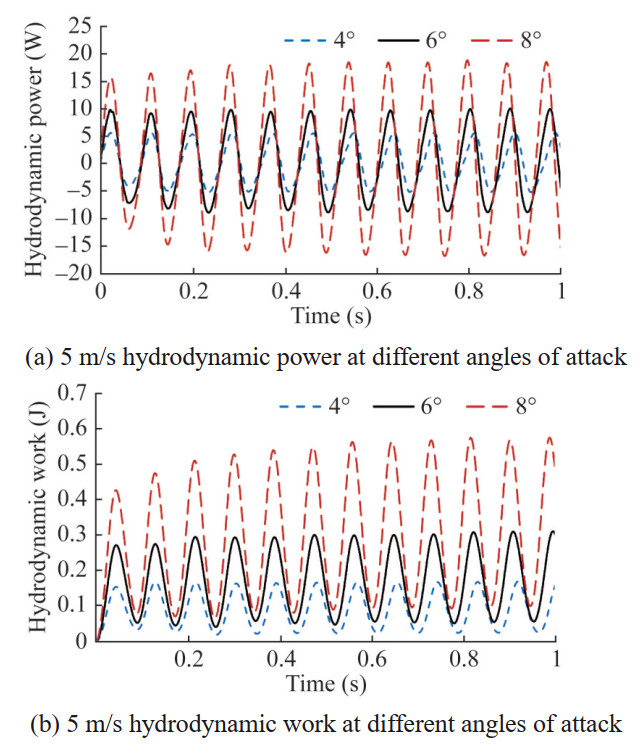Figure  27  Hydrodynamic power and work history results at different angles of attack (5 m/s)

Download: Full-Size Img

The vorticity results of the flow field at angles of attack of 4° and 8° are shown in Figure 28, which also correspond to the last complete cycle of the hydrodynamic power curve.

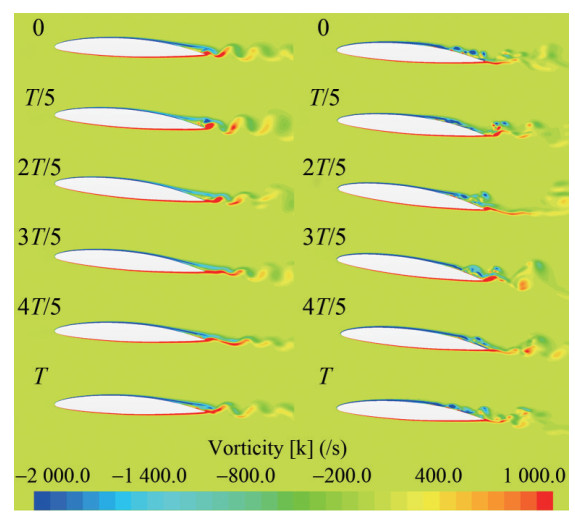Figure  28  Vorticity results of the flow field at different angles of attack (left: 4°, right: 8°)

Download: Full-Size Img

It can be seen that at a 4° angle of attack, the vibration amplitude of the hydrofoil is relatively small, and there is a relatively obvious alternating trajectory of vortices in the wake field. Due to the influence of the hydrofoil motion and incoming flow, the tail vortices in the downstroke are longer and narrower than in the upstroke. At an angle of attack of 8°, the amplitude of the hydrofoil increases, and the vorticity intensity on the suction side increases and moves towards the leading edge. As the hydrofoil vibrates, the characteristics of alternating vortices emanating from the rear become weaker, and the vorticity distribution in the wake field is more finely distributed.

3.3   Influence of frequency ratio and inertia radius on vibration state

Based on the flutter critical velocity of the 6° angle of attack model, the effects of different natural characteristics of the elastic system on the vibration state are compared and calculated. The other parameters remain unchanged, and the heave and pitch stiffness of the elastic axis are adjusted respectively to change the natural frequency ratio f_h/f_θ of the hydrofoil. Keeping the vertical stiffness constant and increasing the pitch stiffness, a hydrofoil model of f_h/f_θ = 0.845 is obtained; Keeping the pitch stiffness constant and reducing the vertical stiffness, a hydrofoil model of f_h/f_θ = 0.707 is obtained. The vibration state, maximum power and average work for each natural frequency ratio are shown in Table 8. The flow-induced response results of hydrofoils with three frequency ratios at a flow velocity of 5 m/s are shown in Figure 29.

Figure  29  Vibration and hydrodynamic force time history results at different frequencies (5 m/s)

Download: Full-Size Img

From the vibration curve, it can be seen that after increasing the pitch stiffness to make f_h/f_θ=0.845, the vibration frequencies of the hydrofoil heave and pitch motions at the initial stage are higher than those of the original model, and then the amplitude attenuates and the vibration frequency decreases. The heave range of lift and torque also decreases, and the equilibrium position of the heave motions decreases.When f_h/f_θ=0.707, due to the decrease in vertical stiffness, the equilibrium position of the hydrofoil's heave motion is lifted up, and the vibration periods at the 2-DOF are increased compared to the original model, the amplitude also shows an attenuation trend. Figure 30 shows that when the model frequency ratio is 0.707 and 0.845, the power amplitude of the hydrodynamic force and the total work it does gradually attenuate, and the vibrations of the two models are in a convergent state. It can be seen that increasing the pitch stiffness can effectively suppress flutter, and when f_h/f_θ approaches 1, reducing the heave stiffness to stagger the heave natural frequencies from the pitch natural frequencies can also improve hydrofoil flutter.

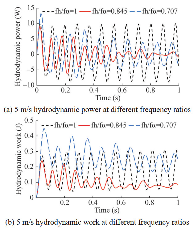Figure  30  Hydrodynamic power and work history results at different frequency ratios (5 m/s)

Download: Full-Size Img

In addition, different structural designs can change the mass distribution of the hydrofoil, thereby changing the inertia radius of the hydrofoil and affecting the inherent characteristics of the system. The following maintains the mass, elastic axis position, stiffness, and centroid position of the hydrofoil unchanged at an angle of attack of 6°. By comparing and calculating the effects of different inertia radii on the flow-induced vibration of the hydrofoil, the dimensionless inertia radius r of the three hydrofoil models are 0.45, 0.542, and 0.634, respectively. The corresponding pure heave frequency f_h is 9.5 Hz, and the pure pitch frequency f_θ is 11.4 Hz, 9.5 Hz, and 8.1 Hz, respectively. The vibration state, maximum power and average work for each dimensionless inertia radius are shown in Table 9. The response results of the three models at a flow velocity of 5 m/s are shown in Figures 31 and 32. It can be seen that when r=0.45 and 0.634, the hydrofoil no longer maintains constant amplitude vibration and exhibits an attenuation trend. The power of fluid work and the energy input for the elastic system significantly decreases with the vibration of the hydrofoil, and when r=0.45, the energy and motion of the system attenuate more rapidly, and the vibration enters a convergent state.

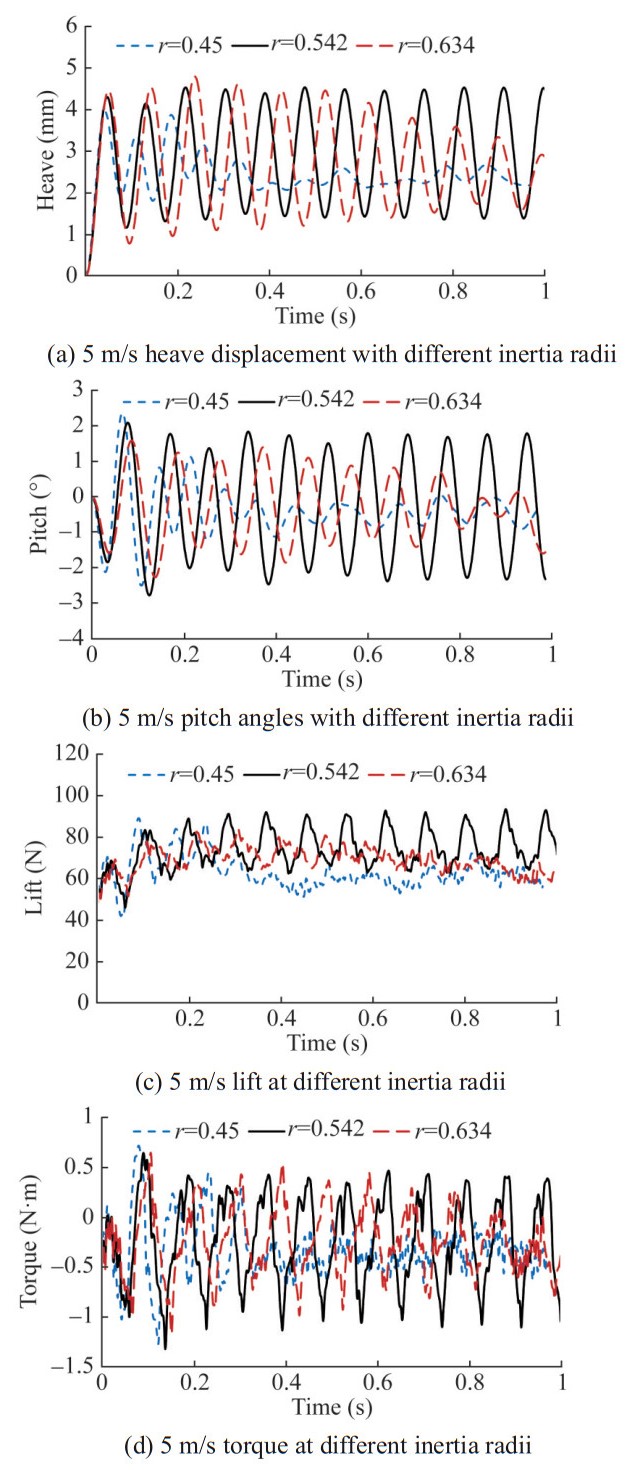Figure  31  Vibration and hydrodynamic force time history results at different inertia radii (5 m/s)

Download: Full-Size Img

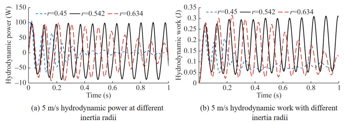Figure  32  Hydrodynamic power and work history results at different inertia radii (5 m/s)

Download: Full-Size Img

The response results of three inertial radius hydrofoils when the flow velocity increases to 6 m/s are shown in Figures 33 and 34.

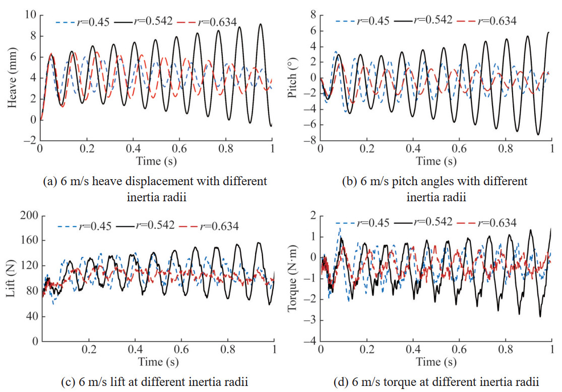Figure  33  Vibration and hydrodynamic force time history results at different inertia radii (6 m/s)

Download: Full-Size Img

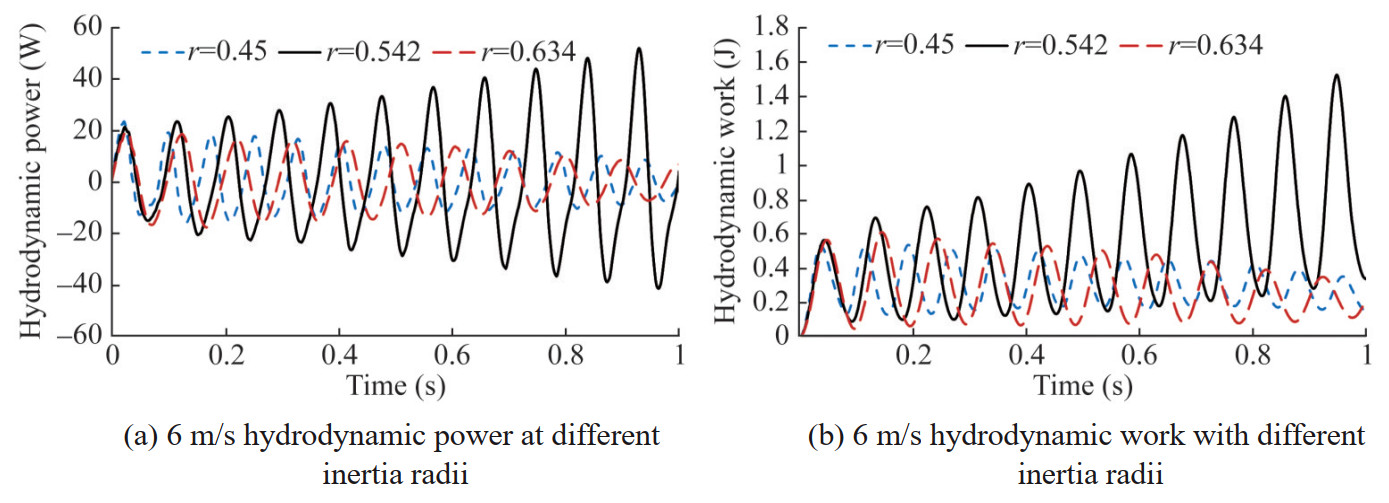Figure  34  Hydrodynamic power and work history results at different inertia radii (6 m/s)

Download: Full-Size Img

At a flow velocity of 6 m/s, the original model (r= 0.542) was already in a flutter state, while the heave and pitch vibrations of the hydrofoil models with r=0.45 and r=0.634 continued to attenuate. The energy input by the fluid to the elastic system gradually decreased, and the vibration remained in a convergent state, but the amplitude significantly increased compared to 5 m/s.

Continue to increase the flow velocity to 7 m/s, and the response results are shown in Figures 35 and 36.

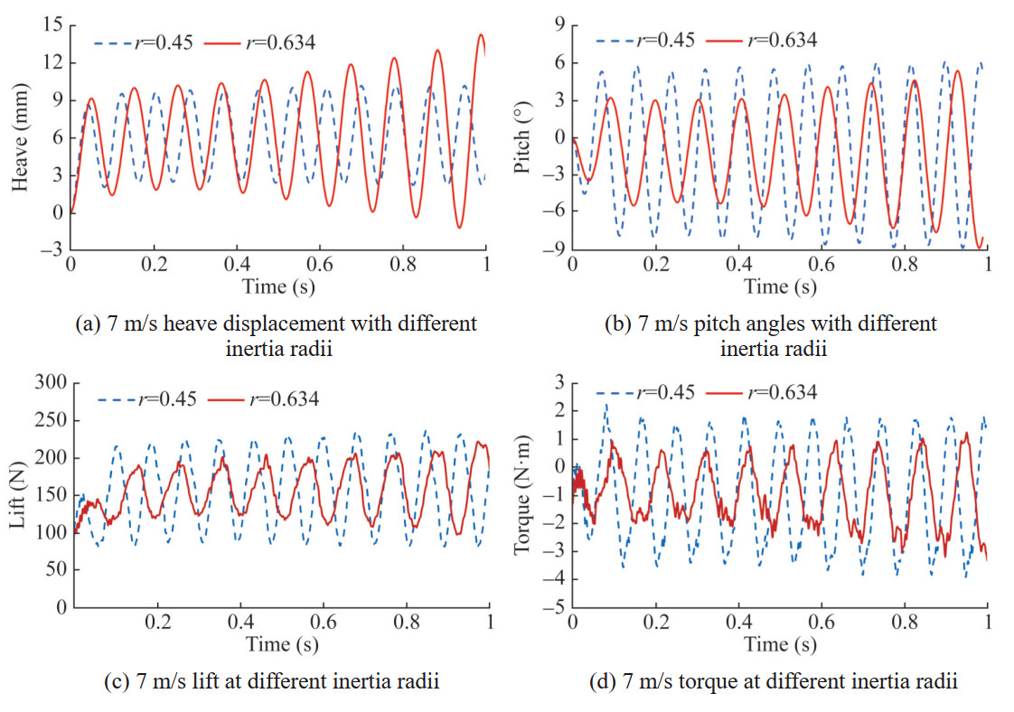Figure  35  Vibration and hydrodynamic force time history results at different inertia radii (7 m/s)

Download: Full-Size Img

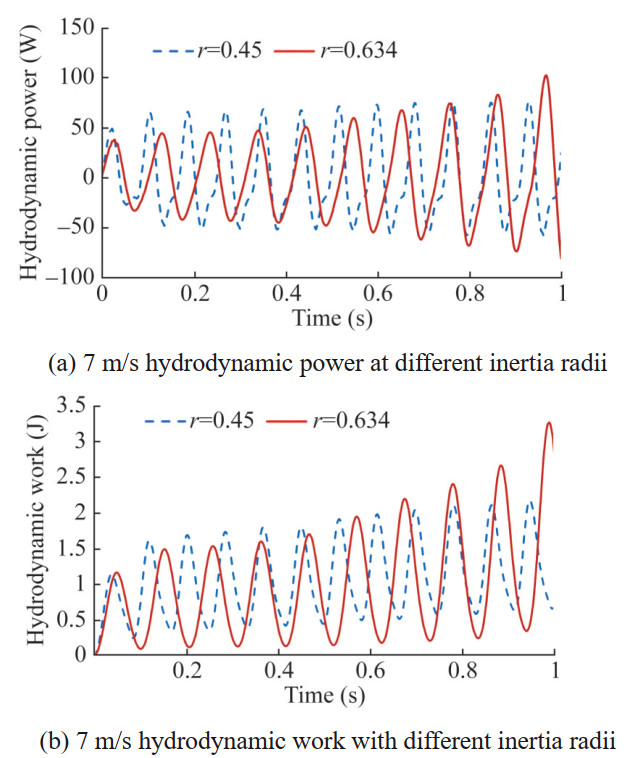Figure  36  Hydrodynamic power and work history results at different inertia radii (7 m/s)

Download: Full-Size Img

At this time, the heave and pitch vibrations of the two models no longer attenuate, and the amplitude increases faster at r=0.634 than at r=0.45. However, due to the larger inertia radius, the vibration period is longer than at r=0.45, and the energy input by the fluid for the two models gradually increases. The hydrofoil enters a flutter state, and the critical velocity increases from 5 m/s to between 6 m/s and 7 m/s. It can be seen that the radius of inertia has a significant impact on the amplitude and frequency of both heave and pitch motions, and can change the critical velocity.

4   Conclusion

Based on computational fluid dynamics and structural finite element methods, a co-simulation framework for the flow-induced vibration of hydrofoil in uniform flow is established and numerical simulation research is carried out. The conclusions drawn from this work can be summarized as follows:

1) The flow velocity has a significant impact on the amplitude of the hydrofoil. The heave and pitch motions at low flow velocity are mainly affected by the second-order natural characteristics of the elastic system, and as the flow velocity increases, vibration begins to be dominated by a single frequency. When the input value of the fluid energy exceeds the dissipation value, the hydrofoil will enter the flutter critical state without amplitude attenuation.

2) The attack angle of the hydrofoil has a significant impact on the vibration amplitude, but has no apparent effect on vibration frequency and critical velocity.

3) Adjusting the natural frequency ratio by reducing the vertical stiffness or increasing the pitch stiffness can move the vibration from a critical state to a convergent state. To increase the critical velocity of the flutter, the natural frequencies of heave and pitch can be staggered by adjusting the inertia radius.

Different geometric shapes will alter the excitation force characteristics of the flow field, thereby affecting the vibration of the hydrofoil. This work mainly calculates and analyzes the vibration characteristics of hydrofoils at different flow velocities and angles of attack, so it is possible to explore the impact of different trailing edge shapes on hydrofoil vibration in the future.