1   Introduction

The underwater acoustic (UWA) channel is recognized as one of the most challenging communication channels due to its adverse time-frequency selectivity, limited bandwidth, and random noise (Jiang et al., 2022; Jiang and Diamant, 2023; Zhu et al., 2023; Zhu et al., 2021; Song et al., 2019). The time variation of the UWA channel is generally coupled with the complicated marine environment at different time scales (Oliveira et al., 2021; Zhou et al., 2015; Yang et al., 2017). For example, the scattering of surface waves may lead to small-scale phenomena. Meanwhile, the sound speed profile, surface height, and the motion of the transmitter/receiver will cause large-scale phenomena (Qarabaqi and Stojanovic, 2013). Substantial research has conducted in the past years, overcoming the impact of the underwater environment and improving the UWA communication quality. A consensus indicates that the throughput and robustness of the UWA communication link will be improved futher if the UWA channel properties are maximized and an adaptive UWA communication method is tuilized.

The quality of channel information, which is feedback from the receiver, determines the performance of the adaptive UWA communication systems. Supported by a proper channel, the adaptive UWA communication system can determine the physical layer parameters and the selected environment match modulation schemes, such as using a low-modulation scheme and spread spectrum technology under the multipath channel. The channel received by the transmitter is frequently outdated due to the slow acoustic propagation and the fast time-varying UWA channel. Therefore, a channel prediction model that does not rely on extra training sequences in the receiver is required.

In terrestrial wireless communication, channel prediction has been widely used in beam-forming, physical security, and fifth-generation usage scenarios. However, in the UWA communication society, the UWA channel prediction has only seen application in recent years. The channel prediction approach can be mainly divided into two categories: model-dependent and model-independent (Liu et al., 2021; Zhang et al., 2020a). The former approach assumes that the previous knowledge of the UWA channel is known, and the prediction performance can thatn be improved when the correctly defined model matches the realistic channel model. The UWA channel evolution in Fuxjaeger and Iltis (1994) was modeled as an autoregressive process, and the channel parameters were predicted by extended Kalman filter because of the assumption of the uncorrelation channel tap and independent transitions. Nadakuditi and Preisig (2004) assumed that the multipath is adopted to optimize the postfiler coefficients for tracking the channel. Thus, the model-dependent approach could attain no more than the comprehensive of the researchers. That is, if the natural UWA channel does not match the assumed model, then the prediction performance based on the model-dependent approaches cannot be effectively presented.

In constrast to the model-dependent approach, the model-independent method disregrads previous knowledge of the channel, such as the adaptive and deep learning channel predictions. This type of approach can track the channel per tap based on the history of channels. The adaptive algorithms, namely the least means square (LMS) and RLS, are widely used to update the channel. Similar to many adaptive processing applications, the RLS has superior accuracy with high computational complexity compared with LMS. A channel prediction network that comprises a one-dimensional convolutional neural network and a long short-term memory (LSTM) model is designed in Liu et al. (2021). However, the existing UWA channel predictor occasionlly considers the inherent physical sparsity and the evolutionary correlation of the UWA channel. A channel prediction model based on LSTM integrated with the attention mechanism is proposed in this paper, and the performance is analyzed under different UWA channels to exploit their characteristics.

The key idea of the attention mechanism comes from the human visual attention mechanism. When peopeo perceive things, they often provide increased attention to specific parts based on their needs. Motivated by this natural phenomenon of humans, the attention mechanism is widely applied in several fields with remarkable results. A recurrent neural network (RNN) using an attention mechanism was proposed by Mnih et al. (2014) in computer vision for image classification. In Bahdanau et al. (2016), an attention machanism with RNN was first used in machine translation work. The attention mechanism can generally be regarded as a resource allocation scheme, which is the primary means to solve the problem of information overload (Niu et al., 2021).

The significant contributions of this paper are presented as follows. A learning model named AttLstmPreNet is designed for UWA channel prediction, which is integrated with an attention mechanism using an LSTM network. The proposed AttLstmPreNet can exploit the sparsity and time evolution of the UWA channel to conduct the channel prediction effectively. The prediction performance was evaluated using a set of simulation channels. Notably, the proposed AttLstmPreNet is a hybrid channel prediction approach between model-dependent and mode-independent because this approach is driven by the history of channel data and the previous knowledge of channel data.

2   UWA channel characteristics

Owing to the physiucal characteristics of the underwater environment, namely the dynamic of the sea environment, the UWA signal will be reflected and scattered, resulting in the receipt of signal along with multiple propagation paths, and this phenomenon is known as the multipath effect. Theoretically, the number of propagation paths was infinite. However, most paths can be ignored with the transmission loss, and a few dominant paths with high energy should be considered; thus, the UWA channel will almost emerge in a sparse structure.

UWA channels can be regraded as a function of time and depth. A coherent function was proposed to describe the temporal coherence of UWA channels (Yang, 2012), which can be expressed as follow:

where the h (t) is the reference estimated channel at geotime t, and h (t + τ) is the channel arriving with a latency τ, [pq] denotes the maximum valued of the correlation between the p and q signal. (·)^* is the conjugation operation, and the $ <\cdot> $ is the ensemble average function over geotime t (Huang et al., 2013). The temporal coherence of the UWA channel was computed in different time scales (i.e., interpacket, intrapacket) under different sea states using Equation (1). The results show that the channel coherence is high during the intrapacket and the interpacket in the calm sea. The correlation of channels is poor under the rough sea. Figure 1 shows the intrapacket temporal coherence under different sea conditions.

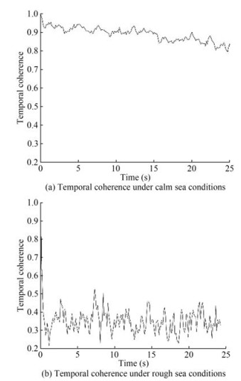Figure  1  Temporal coherence of different UWA channels

Download: Full-Size Img

The following observations can be drawn from the discussion above,

• Most UWA channels have a sparse multipath arrival structure, which is caused by the propagation environment.

• Under different environmental conditions, the evolution of the UWA channel has varying temporal coherence. In particular, the UWA channel exhibits remarkable temporal coherence in stationary environments (such as in a calm sea or protected ocean). By constrast, the temporal correlation of the channel is poor in nonstationary environments (such as in a rough sea or open ocean).

The paper aims to provide an LSTM-based channel prediction model with an attention mechanism to improve adaptive UWA communication by exploiting the channel properties (sparsity and temporal coherence).

3   UWA channle prediction model based on LSTM with attention mechanism

3.1   UWA single-carrier communication system

Consider a single-input-single-output single-carrier acoustic communication system in a dynamic ocean environment. The binary information bit is divided into $P$ groups, in which $P$ denotes the number of bits per symbol, and each group is mapped to one of the $2^P$-ary symbols of the map alphabet $A=\left\{\alpha_p\right\}_{p=1}^P$, where $\alpha_p$ can be a complex or real value. The transmitted symbol vector is constructed by concatenating a training symbol sequence of length $N_t$ with the information symbol sequence. That is, the transmitted symbol vector can be represented as $\boldsymbol{x}=\left\{x_n\right\}_{n=1}^{N_s}$, where the $N_s$ denotes the length of the transmitted symbols.

The transmitted symbols are filtered via a raised-cosine pulse-shaping filter with an impulse response g (t) to form the baseband signal u (t), which can be written as follows:

where g (t) is a raised-cosine pulse-shaping filter with a roll-off factor γ, and T_s is the symbol interval. The passband transmitted signal u (t) is produced by the s (t) modulated with a carrier frequency f_c, namely:

Assume that the channel delay length is L. The received baseband singal is distorted by multipath spread and noise can then be expressed as shown below:

where the h_l (t), τ_l is the time-varying fading factor and delay time corresponding to the lth propagation path, and noise (t) is the equivalent baseband noise at the receiver, which is independetn of the s (t).

The baseband channel information can be estimated by using the knowledge of the transmitted and the received baseband signals, that is, s (t) and y (t). Many scholars have developed UWA channel estimation algorithm in the past years, such as maximum likilihood, least squares, and compressed sensing. Herein, the estimated channel in baseband can be expressed as shown below:

where h_l (t) and τ_l (t) denote the fading amplitude and the time delay of the discrete channel path, respectively.

3.2   Brief review of the UWA channel prediction method

The traditional model-independent channel predictor, such as the LMS and RLS, are highly suited for channle prediction in real-world communicaiton systems (Lin et al., 2015; Ma et al., 2019; Radosevic et al., 2011). The general channel prediction structure can be modeled as follows:

where $l$ denotes the channel tap index corresponding to the time delay, $m$ denotes the channel geotime, $\boldsymbol{w}[m, l]=$ $\left[w_0[m, l], w_1[m, l], \cdots, w_{n-1}[m, l]\right]^{\mathrm{T}}$ represents the prediction coefficients, $\hat{h}[m, 1]=[h[m, 1], h[m-1, l], h[m-$ $2, l], \cdots, h[m-n+1, l]]^{\mathrm{T}}$ represents the estimated value at $l$th channel tap in the historical moment, and $n$ is the order of the predictor.

From the above description of Equation (6), the channel prediction approach works by the per channel tap, implying that the computational complexity rises with the channel length. The channel prediction algorithm can impose several significant channel taps to eliminate the noise perturbation and improve the channel prediction accuracy due to the sparsity of the UWA channel; however, determining the critical channel tap should be carefully studied (Lin et al., 2015; Radosevic et al., 2011).

The goal for adaptive predictor based on LMS or RLS is solving the prediction coefficients w[m, l] of Equation (6). The two approaches are briefly described below. Assuming at the geotime (m − 1)th, the channel prediction error at geotime mth can be computed by the Equation (6) and be written as follows:

In the core idea of LMS, the update of w [m, l] lies in the criterion of the least mean square error, namely the minimization of the cost function $. Thusm the prediction coefficients can be updated below:

where μ is the step size and 0 < μ < 1, which controls the tracking performance of w. According to the Equation (8), the previous coefficients and the past channel information with step size are managed to form the new prediction coefficients. The step size μ must compromise the perdiction performance and convergence speed of the LMS algorithm.

Unlike the LMS prediction algorithm, the goal of RLS is to minimize the sum of the error squares between the actual and predicted value. The cost function can be expressed as $ J_w=\sum\limits_{j=1}^n \lambda^{n-j}|e[m, l]|^2$, where λ is the forget factor 0 < λ < 1, which is used to balanced the old and present data.

The selection of λ should match the emporal coherence of UWA channels. The prediction step of RLS is as follows:

where $e\lfloor m, l\rfloor=\hat{h}\lfloor m, l\rfloor-\boldsymbol{w}^{\mathrm{T}}\lfloor m-1, l\rfloor \hat{\boldsymbol{h}}\lfloor m-1, l\rfloor $ is the prediction error, and k [m − 1, l] is the RLS gain vector:

where the matrix P can be computed by the recursion:

where the P [0, l] = δ^-1 I and δ is a tiny number.

3.3   Proposed UWA channel prediction model

3.3.1   Channel prediction based on LSTM

The LSTM is a variant of an RNN and can solve the problems of exploding and vanishing gradients, which is suitable for time series prediction (Zhu et al., 2021; Zhang, 2020b; Zhang et al., 2019; Greff et al., 2017).

In the application of channel prediction, the channel data (measured from the real world or generated from the UWA channel simulator (Qarabaqi and Stojanovic, 2013)) are applied to train the LSTM model. The update of the well-trained LSTM network for channel prediction can be expressed as follows:

where H_t is the history channels, h_t is the predicted output channel, and W_LSTM is the parameters of LSTM that can be trained. Contatenting LSTM, a regression layer is used to make a regresion of the prediction channel as follows:

where W_reg is the paramters of the regression layer that can be trained.

3.3.2   Attention mechanism

Under the same principle of the attention mechanism, many scholars have developed some modifications and improvements in the attention mechanism for adapting to a specific task. The variants of attention mechanism can be categorized into two types: soft attention, and hard attention, under the softness of attention criterion (Niu et al., 2021). Compared with soft attention, hard attention requires minimal computation because computing all attention weights for all elements is unnecessary. The operation of hard attention can be regarded as making a hard decision for each input and is thus non-differentiable and difficult to optimize (Xu et al., 2015).

On the contraty, soft attention aims to compute the probability for each input sequence element when calculating the attention distribution. Comprehensively, he weights on each element are usually calculated by a SoftMax function, and the output is an operation of weights with an input sequence. The entire computing process can be describeed as a differentiable function (Xu et al., 2015). Thus, the attention mechanism can be trained jointly with the rest of the networking using backpropagation method.

Assuming the input sequences, $ \boldsymbol{X}=\left[\boldsymbol{x}_1, \boldsymbol{x}_2, \cdots, \boldsymbol{x}_N\right]$, x_n = $\left[x_{n, 1}, x_{n, 2}, \cdots, x_{n, L}\right]^{\mathrm{T}} $, and n ∈ [1, N]. For each element of X, the attention mechanism generates a positive weight α_{i, j}, i ∈ [1, N], and j ∈ [1, L]. The weight α_{i, j} is computed by an attention model f_att (⋅) and can be expressed as follows:

where α_{i, j} is the element of α_i. While the refined sequences by the attention mechanism can be written as:

where ⊙ represents element-wise multiplication.

Soft attntion is adopted in this paper. A simple but effective soft attention mechanism is parcticed in the designed mode via a dense connection layer with a Softmax function.

3.3.3   Designed attention LSTM for UWA channel prediction

Following the brief introduction of LSTM and the attention mechanism, a learning model called Attention LSTM is developed for the UWA channel (AttLstmPreNet). Figure 2 shows the full architecture of the proposed networ, which comprises an attention mechanism and LSTM model. The attention mechanism is adapted to focus on the characteristic of the history channels, which are constructed by a dense layer connected with the input of the network.

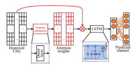Figure  2  Structure of AttLstmPreNet

Download: Full-Size Img

Consider a set of channels $\boldsymbol{H} \in R^{M \times N}$, where $M$ and $N$ denote the geotime and channel tap (i.e., the time delay), respectively. After processing by the attention mechanism, the focused dataset $\boldsymbol{H}^*$ can be computed as follows:

where [α₁, α₂, ⋯, α_N] can be learned from the attention mechanism following Equation (14). An LSTM model is then adopted to predict channels under the learned long-term dependencies. The output channel of the LSTM model can be obtained on the basis of Equation (12) and (13). The attention mechanism can provide corresponding attention to the input channel set with the natural properties of UWA channels. Therefore, the proposed AttLstmPreNet incorporates the advantages of LSTM in the temporal information processing and the benefits of the attention mechanism in the feature selection.

The performance of the proposed AttLstmPreNet is evaluated in Section 4. In paricular, the application of the attention mechanism will be imposed on the following three aspects: channel tap (AttLstmPreNet-Type1), prediction time step (AttLstmPreNet-Type2), and jointly with channel tap and prediction time step (AttLstmPreNet-Type3).

4   Numerical simulation

The performance of the aforementioned channel prediction models, namely, the type of AttLstmPreNet-based, the plain LSTM-based, the LMS-based, and the RLS-based, is compared using the simulation channel measurements. The simulation channel measurement data are generated from the time-varying UWA channel simulator (Qarabaqi and Stojanovic, 2013), which also considers physical aspects of acoustics propagation as the inevitable random channel variations. Zhang et al. (2020a) used the simulator to approximate the real-world channel measurements with different degrees of mobility, such as the Surface Processes and Acoustic Communications Experiment in 2009 (SPACE’08) and the Mobile Acoustic Communications Experiment in 2010 (MACE’10). Two UWA channel measurements were simulated (Cases A and B) in the current study. The system parameters are provided in Table 1 as follows.

4.1   Simulaiton channel analysis

Following Table 1, Figure 3 shows the ensembles of simulated time-varying UWA channels over the measurement duration of 180 s. The vertical and horizontal axes denote the geotime and time delay, respectively. Figure 3 shows that the channel is time-varying, especially in the channel amplitude and delay. Meanwhile, Figure 3 also indicates the sparse structure of the UWA channel. It should be noted that the horizontal axes in Figure 3 represent the time-delay axis with the unit ms, and the vertical axis represents the geo-time axis and its unit is s. Following Equation (1), the temporal coherence of the mentioned simulation UWA channels was computed, as shown in Figure 4. The temporal coherence in Case B is higher than that in Case A, which is consistent with the simulation settings. The similarity definition (Yang, 2012; Zhou et al., 2017; Tu et al., 2021) revealed that the channel whose temporal coherence is larger than 0.85 is defined as a slowly varying channel; otherwise, the channel is fast varying.

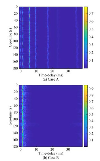Figure  3  Simulation time-varying channel impulse responses

Download: Full-Size Img

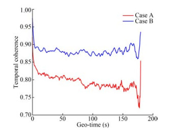Figure  4  Temporal coherence of Case A and Case B

Download: Full-Size Img

4.2   Prediction performance comparison

The aformentioned channel predictors are deployed for training and analysis. All channel predictors were trained on the simulation channel measurements of Cases A and B, comprising 361 samples (80% of the channel set were used for training, and the rest were used for testing). The AttLstmPreNet model comprises attention, LSTM, and dense models, while the plain LSTM is constructed by two LSTM layers and a dense layer. The loss function of the LSTM is the mean absolute error (MAE). All LSTM models were implemented with Keras running on top of TensorFlow, which is performed on a computer with 2.5 GHz Intel (R) Core (TM) i7-11700K CPU (64 G RAM) and Ge-Force GTX 1050 Ti GPU. The prediction order for LMS and RLS channel preditors is set 8. The step size μ of LMS is to set 0.7 and 0.3 for Cases A and B channel sets, respectively. The forget factor λ of RLS is set to 0.85 and 0.75 for Cases A and B channel sets, respectively (the parameter set referenced from Liu et al. (2021). Notably, the parameters of LMS and RLS are empirical values depending on the UWA channel properties. The training loss of the mentioned LSTM-based models in different channel sets is given in Figure 5. The loss value for each model decreased as the training epoch progressed. Figures 5(a) and (b) show that the AttLstmPreNet-Type2 achieves low loss value curves with a faster rate than other LSTM-based models in Cases A and B channel sets, respectively, thereby imposing that the attention mechanism on the time step is beneficial to reducing the training loss. In particular, in the fast time-varying UWA channel set (i.e., Case A), AttLstm-PreNet-Type2 has a faster convergence speed compared with the plain LSTM.

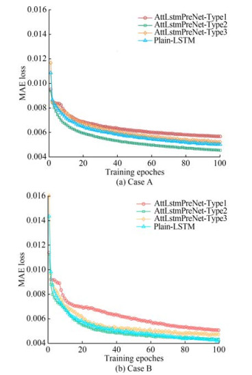Figure  5  MAE loss curve of the mentioned prediction models during the training phase

Download: Full-Size Img

Figures 6 and 7 show the prediction channel by applying the well-trained methods on Cases A and B, respectively, namely AttLstmPreNet-Type1, AttLstmPreNet-Type2, AttLstmPreNet-Type3, plain LSTM, LMS, and RLS. Similar to the training phase, the MAE loss function is used to measure the error of prediction results, as shown in Table 2. From the MAE loss, the mentioned predictors work well in the slow time-varying channels. The RLS predictor achieved lower MAE values among the fast and slow time-varying channels than the LMS predictor. Notably, the parameters of RLS should be finetuned compared with the LSTM-based predictor. For LSTM-based predictors, the AttLstmPreNet-Type2 and AttLstmPreNet-Type3 work slightly better than plain LSTM in different time-varying channels. Considering model simplification, the AttLstmPreNet-Type2 should be encouraged. In a large number of multipath conditions (i.e., Case A), the AttLstmPreNet-Type1 showed similar performance to plain LSTM, while the performance of AttLstmPreNet-Type1 is worse than the plain LSTM in Case B. The result indicates that the AttLstm-PreNet-Type1 is suitable for a channel with more cluster multipath than plain LSTM with a simple structure.

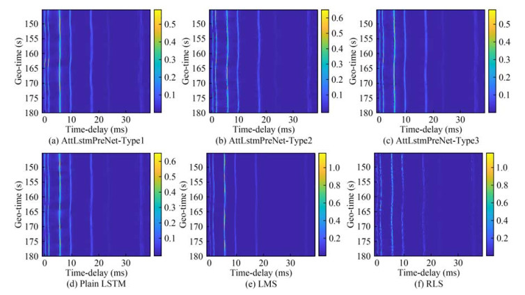Figure  6  Prediction results for Case A using the mentioned predictors

Download: Full-Size Img

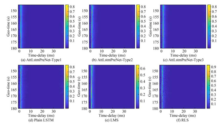Figure  7  Prediction results for Case B using the mentioned predictors

Download: Full-Size Img

5   Conclusions

A deep learning approach is applied in this paper to time-varying UWA channel prediction. A novel deep learning model named AttLstmPreNet is designed on the basis of LSTM with an attention mechanism. In the proposed model, AttLstmPreNet exploits the attention mechanism and LSTM network to capture temporal information from the historical UWA channels. A soft attention mechanism is introduced before the LSTM to support the model to focus on the features of input sequences and help improve the learning capacity of the proposed model. Experimental results on the simulated dataset demonstrate the effectiveness of the proposed model. The results show that the proposed model is better thant the adaptive channel predictors (e.g. LMS or RLS predictor).

The authors believe that this paper is the first to desin an LSTM model with an attention mechanism for UWA channel prediction with a simulation channel dataset. Applying the attention mechanism to real-world UWA communication systems will be an essential issue. Thus, highly advanced attention mechanisms will be introduced in the future. Meanwhile, the parameter optimization of the adaptive channel predictors must be studied jointly with the UWA properties.