1   Introduction

Underwater acoustic (UWA) communications constantly suffer from long delay spread, severe Doppler effects, and time variation (Eggen et al., 2000). These factors are serious obstacles, particularly for high-rate transmission, and must be overcome.

Orthogonal frequency division multiplexing (OFDM) technology has been widely studied in high-rate UWA communication systems because of its high bandwidth efficiency and robustness to multipath delay. However, the rectangular time-domain window used for each subcarrier in OFDM leads to significant out-of-band emission in the frequency domain. Moreover, OFDM systems are susceptible to synchronization errors (Pollet et al., 1995), especially in scenarios with severe Doppler frequency shifts (Morelli et al., 2007), due to the frequency limitations of rectangular time-domain pulses.

Filter bank multicarrier (FBMC) systems with offset quadrature amplitude modulation (OQAM) are highly robust to carrier frequency offsets due to the pulse-forming filters. These systems reduce out-of-band energy leakage and can easily satisfy system synchronization requirements (Pérez-Neira et al., 2016). Furthermore, sharp frequency–time filters (Siohan et al., 2002) used in FBMC-OQAM can minimize intersymbol interference without cyclic prefixing, which is required in OFDM. Thus, FBMC has higher spectral efficiency than OFDM (Saeedi-Sourck et al., 2011). Overall, FBMC-OQAM has a lower out-of-band interference rate (Nam et al., 2016), a flexible bandwidth (He et al., 2019a), better time–frequency focusing characteristics, and higher spectral efficiency than OFDM, making it an excellent candidate modulation method for future communication systems (Nissel and Rupp, 2018).

In OFDM or FBMC-OQAM systems, an accurate channel estimator (CE) is conducive to accurate symbol detection. Especially in time-varying UWA channel environments, channel estimation and tracking are usually necessary. For OFDM systems, multicarrier symbol blocks transmitted at different times do not overlap with each other. Achieving channel tracking by inserting comb-type pilots is easy due to the aforementioned feature. While for FBMC-OQAM systems, pilots are interfered with by unknown symbols around them due to the overlapped multicarrier symbols. In other words, the received pilots in OFDM systems are only affected by the channel, while the received pilots in FBMC systems are further affected by many unknown data symbols. Therefore, the comb-type pilot structure in OFDM systems cannot be directly used for channel tracking in FBMC systems, but the inherent interference of the received pilots must be eliminated or reduced first. The inherent interference lies in the effect of energy leaked by symbols in the time and frequency domains on other symbols after the orthogonality between symbols is lost. Therefore, the traditional channel estimation methods for FBMC-OQAM systems can be divided into two categories: preamble-based methods (Lélé et al., 2008) and scattered pilot-based methods (Javaudin et al., 2003). When all pilots used for channel estimation are placed at the beginning of a signal block, it is called the preamble-based method. When pilots are placed at isolated time–frequency points throughout the frame, it is called the scattered pilots-based method (Kofidis et al., 2013).

The first type of method is preamble-based and aims to set the symbols around the pilot symbols to zero or set the pilot to a specific value to reduce or cancel directly the interference received by the pilot. A two-step preamble-based design is proposed to estimate the carrier frequency offset and frequency-selective channels in MIMO-FBMC/OQAM systems simultaneously (Singh et al., 2018; 2019). A simple and effective method is proposed on the basis of the continuous preamble sequences. Combined with a low-complexity channel estimation method, the scheme considers adequately designed pilot sequences and self-interference. This scheme provides superior performance considering mean square error (MSE) and symbol error rate (Chen-Hu et al., 2018). An extended preamble structure, which exploits symmetric patterns to cancel interference and consider the weight of interference in the symmetric structure as well as the additional interference from the middle of the leading structure, is proposed (Wang et al., 2018). However, the system overhead of such methods is often large.

The second type, which is based on scattered pilots, usually needs to insert auxiliary pilots around the known pilots. The energy leaked to the pilot by the auxiliary pilot and that leaked by other unknown symbols can cancel each other out by setting different values for the auxiliary pilots. A pilot-aided channel estimation method and a pilot design scheme based on a tile-based subchannel mode are proposed. This method reduces interference and improves the channel estimation performance of FBMC-OQAM (He et al., 2012). A three-dimensional pilot-aided channel estimation scheme is proposed for MIMO-OQAM systems with spatially correlated channels. The scheme is based on assigning pilots in three dimensions: time, frequency, and space. The scheme handles the inherent interference of MIMO-OQAM and maximizes spatial channel correlation to reduce the total pilot overhead without degrading the channel estimation accuracy (Kalil et al., 2013). An auxiliary pilot-based method is proposed to reduce the inherent interference on the scattered pilots to improve the channel estimation accuracy (Fuhrwerk et al., 2017). When used for continuous tracking of time-varying channels, the pilots and auxiliary pilots can be arranged into a comb-type structure, which is similar to the comb-type pilot in OFDM systems. The overhead of the second type is less than that of the first type. However, the overhead is still relatively large for the UWA channel with a long delay.

Preamble- and scattered pilot-based methods constantly assume that the symbol duration is substantially longer than the maximum channel delay. The performance of these channel estimation schemes degrades significantly when the assumptions are unsatisfied (Cheng et al., 2019a).

Deep learning (DL), known for its powerful learning and recognition and prediction capabilities, has also been introduced into communication systems to obtain superior performance in time-varying channel estimation (O'Shea and Hoydis, 2017). Support vector machines are extended from the earliest classification problems to regression estimation problems (Vapnik et al., 1996). A nonlinear complex support vector regression approach is proposed and applied to the auxiliary pilot-based FBMC-OQAM channel estimation problem. The algorithm first obtains a learning model from the least square (LS) pilot estimates and then predicts the channel estimates of other subcarriers by this model (He et al., 2019b). A channel estimation and equalization scheme based on deep bidirectional long short-term memory networks was proposed in 2019 (Cheng et al., 2019b). In the same year, they also took the channel estimation and equalization problem in FBMC systems as a DL task and proposed a DL-based channel estimation and equalization scheme for FBMC systems. Channel estimation and equalization and QAM demapping are treated as black boxes in their model, and their roles are continuously approximated by a DNN model. However, DL-based methods often require high computational complexity.

The sparsity of the UWA channel can reduce the complexity of channel estimation (Li and Preisig, 2007). Shallow water surface scattering channels have a sparse structure at sufficiently wide bandwidths. This structure is formed by multipath arrivals resolved in delayed form (Li, 2006). A sparse adaptive subspace tracking (SASP) method is proposed to improve the accuracy of LS channel estimation. Two channel frequency response estimation algorithms, namely auxiliary pilot SASP and code-SASP, are proposed for FBMC-OQAM systems (He et al., 2019b). A Bayesian learning-based sparse channel estimation technique is proposed for quasi-static and doubly-selective mmWave hybrid MIMO-FBMC systems. In contrast to the interference approximation method model, the proposed time-domain sparse Bayesian learning (TD-SBL) scheme can successfully estimate frequency-selective channels strongly (Srivastava et al., 2020; Singh et al., 2022). A low-complexity algorithm, namely a dynamic threshold-based inner product operation optimization strategy for MIMO sparse channel reconfiguration, is proposed for MIMO-FBMC sparse channels to reduce complexity (Wang et al., 2020). The block SBL algorithm is introduced to improve the channel estimation performance using the block-sparse structure of the sparse multipath channel model (Wang et al., 2021). A sparse channel estimation method for MIMO FBMC-OQAM systems, which can achieve accurate channel estimation by adaptively selecting the support set, is introduced (Wang, 2018).

In short-range high-rate UWA communication scenarios, the sparsity of the UWA channels may not be observed, and reducing the system complexity and overhead is difficult. However, obtaining high signal-to-noise ratio (SNR) signal blocks is easy for the receiver in the case of short distances. This paper studies the channel tracking algorithm based on the data reuse method to meet the requirements of high-speed UWA in this scenario.

The data reuse-based time-varying channel tracking method is a mature technology in conventional OFDM and single carrier systems. Compared with pilot-based methods, the data reuse-based method needs low system overhead. The basic idea is to detect the current data symbols according to the historical channels and then use the detected data symbols as new pilots to update the current channel to achieve channel tracking. For conventional OFDM systems, these data symbols can be used for channel tracking as long as the length of the cyclic prefix or guard interval is longer than the channel delay and the Doppler and residual frequency offset are well compensated. The problem of inherent interference must be overcome to apply the data reuse technology to FBMC-OQAM systems. This problem can be divided into two subproblems: detection of the interference source symbols and iterative updating of the channel after interference elimination from the reused symbols.

The innovative contributions in this paper are described as follows to solve the two aforementioned problems.

1) A time-varying UWA channel input–output model for FBMC-OQAM systems based on the unified transmission matrix (UTM) model is established. The time-invariant channel-based UTM model was proposed in a previous work (Lu et al., 2022) to describe the input–output channel relationship of the UWA FBMC-OQAM system. The UTM model in this paper is extended to time-varying channel scenarios without changing the model framework. An efficient symbol detection model based on time-varying UTM is derived. The characteristic of the UTM model lies in its comprehensive and independent description of the weight value of each inherent interference. Therefore, the symbol detector based on the UTM model can realize the unified detection of all interference source symbols.

2) A data reuse-based time-varying channel tracking algorithm for UWA FBMC-OQAM systems with long signal blocks is proposed. This algorithm utilizes an iterative verification method to reduce the impact of data detection errors on channel tracking accuracy. The conventional FBMC-OQAM detector cannot detect all interference source symbols uniformly. Therefore, suppressing the inherent interference of symbols to be reused is difficult, and the data symbols cannot be selected as new pilots for channel tracking. This paper maximizes the advantage of the UTM model, which can detect all interference symbols uniformly. Therefore, the data reuse method can be applied in UWA FBMC-OQAM systems.

The relationship between channel tracking accuracy and channel time coherence of the proposed method is discussed by simulation in this paper. The influence of data detection error on channel tracking error is analyzed. Compared with traditional methods based on known pilots, the proposed method has similar channel estimation accuracy but requires low overhead. The sea trial results further prove the practicability of this method in the application of high-speed UWA communication in short-range and high SNR scenarios. Finally, the results confirmed that the proposed time-varying channel tracking algorithm in this paper is suitable for the high-rate FBMC-OQAM UWA communication applications under the condition of short-range and high SNR.

2   System model

This section first introduces the FBMC-OQAM transmission signal model. Next, the input–output channel model over UWA time-varying channels is derived. Afterward, the extended UTM model is presented to describe the derived input–output channel model. Simplifying the expression of the time-varying channel model in a matrix form is easy by using the UTM model. Therefore, computational complexity is reduced by dividing and solving the model in the form of sub-UTM models. The derivation in this section lays a theoretical basis for channel estimation and symbol detection in Section 3.

2.1   FBMC-OQAM transmitting signal model

An FBMC-OQAM communication system with M subcarriers and N multicarrier symbols is considered in this study. The real and imaginary parts of a complex data symbol are transmitted at staggered T/2 time. The baseband transmission signal can be expressed as

where s_{m, n} is the (m, n)th transmitted real value symbol, T is the transmission interval of adjacent complex data symbols, and g (t) is the prototype filter function. The additional phase rotation of each real value symbol is expressed as ϕ_{m, n} = π (m + n)/2 + mnπ to maintain the real orthogonality between adjacent symbols. The PHYDYAS filter designed by Bellanger et al. (2010) is adopted in the current study. The time-domain expression of g (t) is defined as

where $\mathcal{B}=4, G_1=0.97196, G_2=\sqrt{2} / 2$, and G₃ = 0.235 147. Eq. (2) shows that the period of the prototype filter g (t) is 4T, but the transmission interval of adjacent multicarrier symbols is T/2. Therefore, the FBMC-OQAM multicarrier symbols overlap each other in the time domain, as shown in Figure 1.

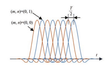Figure  1  Overlapped adjacent multicarrier symbols

Download: Full-Size Img

The passband transmission signal can be expressed as

where Re{·} represents the real part extraction operation and f_c is the center frequency.

2.2   Underwater acoustic channel input – output model for FBMC-OQAM

The time-varying underwater acoustic channel impulse response (CIR) is defined as

where $\tilde{h}_k(t) $ and τ_k (t) are the time-varying amplitude gain and the delay of the kth path of the underwater acoustic channel, respectively. K is the number of channel multipaths. The current study provides the following two approximations to c (t, τ).

Assumption 1: In shallow water environments, the Doppler spread factor of different multipath signals is approximately equal when the communication distance is far larger than the water depth.

Assumption 2: The transmitter and receiver are moving at a relatively uniform speed within the duration of a signal block; that is, the Doppler factor is time-invariant within a signal block.

Then,

where α = v/v_a is the time-invariant Doppler factor. v is the relative speed between the transmitter and the receiver. v_a is the acoustic speed. The received signal $\tilde{y}(t) $ is the convolution of the transmitted signal $\tilde{x}(t) $ and the channel c (t, τ).

where $\tilde{w}(t) $ is the passband additive noise.

The resampling method is employed for Doppler compensation:

where $\hat{\alpha} $ is the estimated Doppler factor. The baseband received signal y (t) when $\hat{\alpha} $ = α can be written as

where w (t) is the baseband noise corresponding to $\tilde{w}(t) $. Eq. (8) shows that the equivalent baseband channel is the sampling of the actual passband CIR after resampling in the presence of a Doppler in the system. The demodulated baseband symbol is expressed as

2.3   UTM model

Equation (9) is the continuous time expression of the input and output model of FBMC-OQAM signal over time-varying UWA channels. The discrete expression of (9) must be further derived to facilitate computer simulation.

Assume that the signal bandwidth is B, and the time sampling interval before upsampling is Δt = 1/B. The relationship between the transmission interval T of adjacent complex symbols and the number of subcarriers M is M = TB. Therefore, t and τ_k in (9) can be replaced by discrete index l and k, respectively. The integral of time can be replaced by the summation of l. As described in Section 2.2, the equivalent baseband channel is the sampling of the actual passband CIR after resampling in the presence of Doppler in the system. Assume that the baseband equivalent channel is $h_k(t)=\tilde{h}_k(t /(1+\alpha)) $. Let $ L=\mathcal{B} M=4 M$, representing the baseband sampling points of the prototype filter.

The discrete expression of z_{m^′, n^′} can then be written as

where w_{m^′, n^′} is the resulting additive noise on the (m, n)th received symbol. The contribution weight Γ_{m, m}^{m′, n′} is specifically expressed as

where $\phi_{\Delta}=\phi_{m, n}-\phi_{m^{\prime}, n^{\prime}}$, and $h_k(l)$ represents the value of the $k$ th tap of the channel at time $l$. Herein, variable $K$ is continuously used to represent the number of channel taps. Some values of $h_k(l)$ are close to zero when the channel is sparse.

The sending symbol $s_{m, n}$, receiving symbol $z_{m^{\prime}, n^{\prime}}$, contribution weight $\Gamma_{m, n}^{m^{\prime}, n^{\prime}}$, and noise $w_{m^{\prime}, n^{\prime}}$ are recombined as shown below to describe (10) in matrix form.

where

Matrix T is the UTM, and (12) is the UTM model. T comprises M × M submatrices Λ_m^m', which are composed of N × N scalar elements, that is,

2.3.1   UTM model for time-invariant channel

Submatrix $\boldsymbol{\varLambda}_m^{m^{\prime}}$ describes the contribution weight of $N$ symbols at different times on the $m$ th subcarrier to the symbols on the $m^{\prime}$ th subcarrier. The values of $m$ and $m^{\prime}$ are fixed when the elements in $\boldsymbol{\varLambda}_m^{m^{\prime}}$ are calculated by Eq. (11). Furthermore, the values of $n$ and $n^{\prime}$ are equal when calculating the elements on the main diagonal of $\boldsymbol{\varLambda}_m^{m^{\prime}}$. If the channel is time-invariant, then $h_k(l)=h_k$. Thus, the element values on the main diagonal of $\boldsymbol{\varLambda}_m^{m^{\prime}}$ are equal. However, the element values on the main diagonal of different submatrices $\varLambda_m^{m^{\prime}}$ are different due to varying values of $m$ and $m^{\prime}$. That is to say, the modulus of the elements on the main diagonal of matrix $\boldsymbol{T}$ presents a ladder-like change, and its envelope follows the frequency domain response characteristics of the channel.

2.3.2   UTM model for time-variant channel

Different from the case of time-invariant channels, $h_k(l)$ changes with $n$ and $n^{\prime}$ under time-varying channel conditions. Therefore, the value of the main diagonal elements of $\boldsymbol{\varLambda}_m^{m^{\prime}}$ also changes with $n$ and $n^{\prime}$. The channel temporal coherence function (Yang, 2012) is defined to describe the correlation between channels at different times.

where the angular brackets $ \langle a b\rangle$ denote the maximum value of the correlation between the a and b series. E[·] denotes ensemble average over the geotime t.

2.3.3   MMSE-based symbol detector for FBMC-OQAM under UTM model

In an FBMC-OQAM system, the symbol on one subcarrier only interferes with itself and the symbol on two adjacent subcarriers. Therefore, the UTM presents block diagonalization. A sliding window with a dimension of 3N × 5N is used to segment the UTM and solve the model. This segmentation solution can reduce the overall computational complexity. According to the model described by (12) and (13), the sub-UTM model is expressed as

where

The value range of $p$ is $[1, M-1]$. In particular, when $p=1$, the first $N$ columns of $\boldsymbol{T}_p$ and $\boldsymbol{s}_{p-2}$ are removed in $\boldsymbol{S}_p$; when $p=M-1$, the last $N$ columns of $\boldsymbol{T}_p$ and $\boldsymbol{s}_{p+2}$ are removed in $\boldsymbol{S}_p$.

Next, the real and imaginary parts of the elements in (16) are separated and rearranged. $\boldsymbol{S}_p$ is a real value vector; thus, its imaginary part is zero, and the following can be obtained:

where

and

The dimension of matrix $ \overline{\boldsymbol{T}}_p$ is 6N × 5N when p is 2–(M−2). When p = 1 or p = M − 1, the dimension of matrix $ \overline{\boldsymbol{T}}_p$ is 6N × 4N. MMSE-based detectors can then be applied for symbol detection.

where $\bf{I}$ is the unit matrix. When $p=1$ or $p=M-1$, the dimension of $\bf{I}$ is $4 N \times 4 N$; otherwise, the dimension of $\bf{I}$ is $5 N \times 5 N . \boldsymbol{C}_{\bar{\boldsymbol{W}}_p}$ is the covariance matrix of the resulting noise $\overline{\boldsymbol{W}}_p$.

Finally, all detection results of $\hat{\boldsymbol{S}}$ are obtained by updating the value of $p$.

3   Time-varying channel estimation method for FBMC-OQAM

The analysis in Section 2 shows that the UTM model can adapt to the cases of time-varying UWA channels. That is, the value of the CIR h_k (l) is taken at each time sampling point l into (11) to calculate $ \Gamma_{m, n}^{m^{\prime}, n^{\prime}}$. However, obtaining a considerable amount of unknown channel information remains a challenge. An effective approximate method is necessary to estimate the CIR when n^′ = {0, M/2, M, ⋯, (N−1) M/2} and obtain the channel responses at other times through interpolation.

This section describes the proposed time-varying CIR estimation method for FBMC-OQAM systems. The method is divided into two steps: initial channel estimation and channel tracking. Figure 2 shows the block diagram of the proposed time-varying channel estimation method for FBMC-OQAM systems. The rest of this section will elaborate on this method.

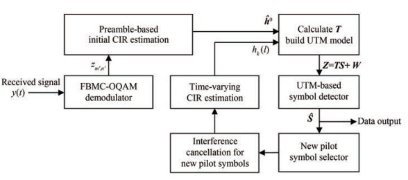Figure  2  Block diagram of time-varying channel estimation algorithm

Download: Full-Size Img

3.1   Initialize channel estimation

Half of the symbols in the preamble are used as pilot symbols to initialize the channel estimation. Figure 3 shows the symbol distribution structure in one FBMC-OQAM signal block. Each circle represents a baseband symbol. Hollow, solid, and crossed hollow circles denote zero, pilot, and data symbols, respectively. The crossed hollow circles with gray background denote the new pilots selected for channel tracking. The dotted line box with blue background is the preamble.

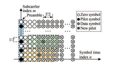Figure  3  Block structure of the FBMC-OQAM signal block

Download: Full-Size Img

According to the time-frequency characteristics of the PHYDYAS prototype filter (Bellanger et al., 2010), the received symbol $z_{m^{\prime}, n^{\prime}}$ is interfered with by the surrounding symbol $s_{m, n}$, where the subscript $m \in\left\{m^{\prime}-1, m^{\prime}, m^{\prime}+1\right\}$ and $n \in\left\{n^{\prime}-3, n^{\prime}-2, \cdots, n^{\prime}+3\right\}$. A protection gap of $3 T / 2$ is set after the preamble to avoid unknown interference with pilot symbols.

Consequently, the UWA channel is the only source of interference with the pilot symbols. Assuming that the channel is approximately time-invariant during the preamble period, (10) can be simplified as

where $ m^{\prime} \in\left\{p_1, p_2, \cdots, p_{M_p}\right\}$, and M_p is the number of pilots. p₁ represents the index of the subcarrier corresponding to the first pilot. The matrix form of the channel estimation model is

where $\boldsymbol{z}_0^{\text {pilots }}=\left[z_{p_1, 0}, z_{p_2, 0}, \cdots, z_{p_{M_p}, 0}\right]^{\mathrm{T}}, \boldsymbol{h}^0=\left[h_0, h_1, \cdots, h_{K-1}\right]^{\mathrm{T}}$, and $\boldsymbol{\psi}=\left[\boldsymbol{\psi}_0, \boldsymbol{\psi}_1, \cdots, \boldsymbol{\psi}_{K-1}\right]$. The superscript 0 of $\boldsymbol{h}^0$ represents the CIR vector when $n^{\prime}=0 . M_p$-dimensional column vector $\boldsymbol{\psi}_k=\left[\psi_{p_1}^k, \cdots, \psi_{p_{M_p}}^k\right]^{\mathrm{T}}$. The calculation expression of the element of $\boldsymbol{\psi}_k$ is

The weighted least squares (WLS) channel estimation can then be expressed as

$\boldsymbol{C}_{\boldsymbol{w}^{\text {piots }}} $ represents the covariance matrix of noise w^pilots. The superscript [·]^T and [·]^H denote transpose and conjugate transpose, respectively.

3.2   Time-varying channel tracking

The channel is time-varying; thus, the accuracy of $\hat{s}_{m^{\prime}, n^{\prime}}$ estimated by $\hat{\boldsymbol{h}}^0$ gradually decreases with the increase of $n^{\prime}$. Therefore, the proposed channel tracking method only uses $\hat{\boldsymbol{h}}^0$ to estimate the data symbols $\hat{s}_{m^{\prime}, n^{\prime}}$ with $n^{\prime}=$ $\{4, 5, 6, 7\}$ and discards the symbols when $n^{\prime}>7$. Symbols with $n^{\prime}=\{1, 2, 3\}$ are zeros. The estimated data symbols are then reused as new pilots to estimate the CIR when $n^{\prime}=4$, i.e., $\hat{\boldsymbol{h}}^4$. Next, $\hat{s}_{m^{\prime} n^{\prime}}$, with $n^{\prime}=\{4, 5, 6, 7, 8\}$, can be estimated by updating $\hat{\boldsymbol{h}}^4$ to (11) and (12). Verifying the detection symbols is necessary due to the presence of possible detection errors of data symbols. The specific method is to redetect $\hat{s}_{m^{\prime}, n^{\prime}}$ with $n^{\prime}=\{4, 5, 6, 7\}$ after updating the estimated $\hat{\boldsymbol{h}}^4$ to (11) and then check the presence of detection errors in $\hat{s}_{m^{\prime}, n^{\prime}}$ If an error exists, then the wrong reused symbol is replaced and $\hat{\boldsymbol{h}}^4$ is reestimated, iterating several times until the estimated value of $\hat{\boldsymbol{h}}^4$ stabilizes. The channel and data symbols at each time can be estimated step by step with this method. The algorithm flowchart is shown in Figure 2.

The temporal coherence coefficient Θ(τ) defined in (15) is used as a measure of channel time variability. A small coherence coefficient indicates a low estimation accuracy. Assuming that when the channel has not excessively changed, that is, the symbols received at the time within the yellow background dotted box, as shown in Figure 3, can be correctly estimated, utilizing these correctly estimated symbols as new pilots for CIR tracking is proposed. The channel error correction code is used to reduce the impact of the time-varying channel. Another important assumption is presented in this paper.

Assumption 3: In the $ {}^{7}\!\!\diagup\!\!{}_{2}\;T$ time range, the unknown data symbols in this range can still be demodulated correctly when the channel is regarded as time-invariant.

UWA channels are often sparse; thus, only a few pilots are necessary to achieve channel tracking and estimation. The sparsity of the channel can be determined in accordance with the estimation results of the initialized channel. K_c is defined as the number of non-zero channel taps, and M_c new pilots are selected for updating the estimated UWA CIR, where K_c < K and M_c > K_c.

According to the block structure shown in Figure 3, the symbols with n^′ = {1, 2, 3} are all zero symbols, which are used to reduce the inherent interference on pilot symbols. Therefore, $\hat{\boldsymbol{h}}^4 $ is the next CIR that must be updated. If symbol s_{m^′, 4} is selected as one of the new pilots to estimate $\hat{\boldsymbol{h}}^4 $, then the subcarrier index of these new pilots can be expressed as a set $ m^{\prime} \in \boldsymbol{\mathcal{S}}_c=\left\{p_1, p_2, \cdots, p_{M_c}\right\}$. Interference cancellation is then performed on the received new pilot symbols $Z_{m^{\prime}, 4}^{\text {pilot }} $; that is,

where $m \in\left\{m^{\prime}-1, m^{\prime}, m^{\prime}+1\right\}, \quad n=\left\{n^{\prime}-4, \cdots, n^{\prime}+4\right\}$, and $(m, n) \neq\left(m^{\prime}, n^{\prime}\right)$. Take $\hat{\boldsymbol{h}}^0$ into (11) to calculate $\Gamma_{m, n}^{m^{\prime}, n^{\prime}}$ in (26). The updated channel pulse response $\hat{\boldsymbol{h}}^4$ is then estimated in accordance with the steps of (23) to (25). Compressed sensing methods, such as orthogonal matching pursuit (Berger et al., 2010), can be used to estimate $\hat{\boldsymbol{h}}^4$ due to the sparsity of UWA channels.

Afterward, $\hat{\boldsymbol{h}}^4$ is taken into (11) and (24) to calculate $\Gamma_{m, n}^{m^{\prime}, n^{\prime}}$ and $\boldsymbol{\varPsi}$, respectively, and $\hat{\boldsymbol{h}}^5$ can be estimated thereafter. By contrast, the CIR at each time is estimated.

4   Simulation and experiment

The analysis in Section 3.2 assumed that the unknown data symbols in this range can still be detected correctly when the time-varying channel is regarded as time-invariant in several FBMC symbol periods. Assumption 3 holds due to the minimum channel temporal coherence coefficients obtained through computer simulation analysis in this section. The performance of time-varying channel tracking in a long FBMC-OQAM signal block is also verified in this paper through simulation and sea trial.

4.1   Simulation

4.1.1   Simulation parameter configuration

The UWA channel simulation model proposed by Qarabaqi (Qarabaqi and Stojanovic, 2013) is adopted. The model of Qarabaqi controls the time variation of the channel by adjusting different channel parameters, such as the position fluctuation of the transceiver affected by the current, the fluctuation of the surface wave, and the change of the scattering. The main parameters and their values set in the simulations are listed in Table 1.

Among the parameters listed in Table 1, the values of Doppler and four large-scale parameters have different effects on channel time variation. Large-scale parameters have considerable influence on the time variation of multipath amplitude and phase, while Doppler parameters have a remarkably significant influence on the time variation of multipath delay. A set speed range of 0–0.4 m/s indicates low-speed movement, and the generated time-varying channel multipath delay does not change within an FBMC signal block period. Meanwhile, a set speed range of 1–3 m/s indicates high-speed movement, and the generated time-varying channel multipath delay will change within a signal block period.

An FBMC-OQAM signal block with M = 128, N = 30, and 3 000 Hz bandwidth is generated in this section for simulation and analysis. The number of symbols N is set as 30, which indicates that the signal is a long signal block. The signal bandwidth is consistent with the simulated channel bandwidth. According to the above parameters, the calculated time period of one FBMC-OQAM multicarrier symbol is 4M/3 000 ≈ 170.67 ms, and the duration of the entire FBMC-OQAM signal block is (0.5MN + 3.5M)/3 000 ≈ 789.33 ms.

4.1.2   Simulation results and analysis

In addition to the main parameters listed in Table 1, the model of Qarabaqi also contains some random parameters, such as the phase of the sea surface wave. Therefore, each generated channel will have slight differences in multipath amplitude, phase, and delay, but their statistical values are unchanged.

An example of the simulated time-varying UWA CIR is shown in Figure 4(a), which demonstrates four main non-zero taps. According to their delay index from small to large, the four main non-zero taps correspond to the direct path, the sea bottom reflection path, the two overlapped bottom surface reflection path, and the twice surface reflection path. The propagation delay of the single surface reflection path is approximately equal to that of the direct path, overlapping to form the first main non-zero tap due to the shallow deployment depth of the transceivers. Moreover, the channel is approximately symmetric due to the depth of the transmitter, and the receiver is similar. Therefore, the channel has two paths with similar delays, and their energy is superposed, corresponding to "Path 2" in Figure 4(a). The relative positions of the transmitter and receiver slightly change in a signal block time period; the delay of the four paths hardly changes. Accordingly, the positions of the four main non-zero taps remain unchanged, while their amplitudes change slightly and continuously. Figure 4(b) shows the time-varying phase of four main non-zero taps. The sea surface is fluctuating, and the sea bottom is stationary. Thus, the phase and amplitude of the twice surface reflection paths (path 3) are highly volatile with time.

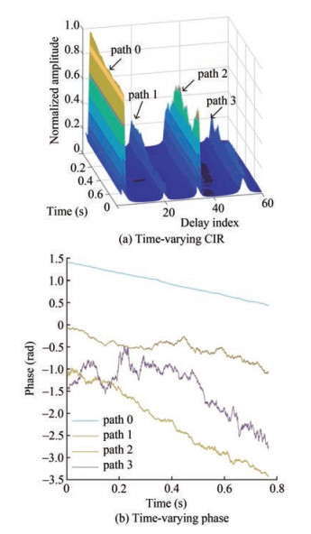Figure  4  Simulated channel based on the proposed model by Qarabaqi and Stojanovic (2013)

Download: Full-Size Img

Figure 5 shows the temporal coherence function of the channels in Figure 4 to measure the time variation of the channel quantitatively. Figure 5 reveals that the channel coherence coefficient decreases to approximately 0.825 within the duration of the entire FBMC-OQAM signal block. The SNR under this channel is set to 20 dB. If only $\hat{\boldsymbol{h}}^0 $ is used for symbol detection of the entire signal block, then the detection result is obtained as shown in Figure 6(a). With the increase of n, the difference between channels at different times rises, which leads to a decrease in symbol detection accuracy. If the method in Section 3.2 is used for channel tracking, then the tracked time-varying channel is taken into the UTM model (18), and the symbol detection results can be improved, as shown in Figure 6(b). The scattered points in Figure 6(b) do not diverge with the increase of n. This result shows that tracking estimation of time-varying channels reduces the bit error rate (BER) of FBMC-OQAM systems with long signal blocks.

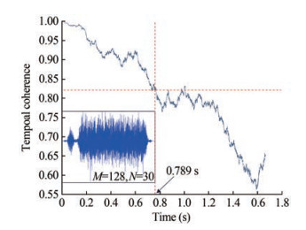Figure  5  Temporal coherence functions of the simulated UWA channels

Download: Full-Size Img

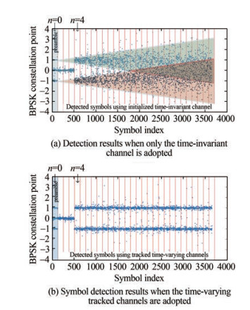Figure  6  Scatter plots of detected symbols when SNR is equal to 20 dB when use different channels

Download: Full-Size Img

The tracking accuracy of the time-varying channel is described by the MSE of channel estimation. The MSE is defined as

The CIR is mainly related to the following factors: the position and velocity of the transmitter and receiver, water depth, sea surface wave, interface reflection coefficient, sound speed, and water reflector or scatterer. In most cases, changes in the position and velocity of the transmitter and receiver, as well as the sea surface wave, significantly impact the channel pulse response within a period of the FBMC-OQAM signal block. Therefore, the attenuation rate of the channel temporal coherence function is adjusted by modifying the simulation parameters, and the performance of the proposed channel tracking method is then analyzed. The MSE results of channel estimation under different SNRs are displayed in Figure 7.

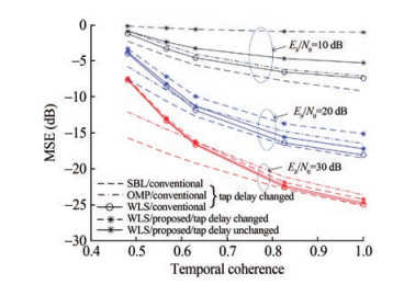Figure  7  MSE of channel tracking error under different SNRs

Download: Full-Size Img

The solid lines with star markers in Figure 7 show that only the amplitude and phase of the tap are time-varying while the tap delay remains unchanged, which corresponds to the relative static or low-speed movement of the transceiver. The dotted lines with star markers indicate that the time delay of the tap is also time-varying, corresponding to high-speed motion. These results show that the channel tracking error decreases with the increase in temporal coherence. Under high SNR conditions, the change in multipath tap delay will not cause substantial performance loss on the proposed method. However, the change in tap delay will markedly reduce the channel tracking accuracy under low SNR. This phenomenon is attributed to the increase in symbol detection error and the difficulty in convergence under low SNR. In addition, Figure 7 shows that the channel tracking performance based on the traditional scattered pilot structure is compared. The conventional method based on known scattered pilot shows high channel tracking accuracy, especially in the case of low SNR, using the WLS-based CEs. The conventional method is unaffected by the data detection error. The CE based on the SBL method shows the best performance, but its computational complexity is also the highest. The CE based on orthogonal matching pursuit (OMP) with low computational complexity is suitable for sparse channels and shows good performance in the case of low channel time coherence. In the case of high SNR and a larger channel time coherence coefficient than 0.8, the channel estimation performance of the proposed method is generally similar to that of conventional methods. However, the system overhead is substantially small.

Figure 8 shows the change of data symbol detection error with SNR. The curves with different markers in Figure 8 correspond to different times of iterative verification. The movement speed of the transceivers in the simulation is set to a random value between 1 and 3 m/s. The tap delay of multipath is time-varying. The WLS-based CE is adopted. The analysis of the results in Figure 8 reveals that the data detection error decreases as the number of iterations increases. The first three iterative verifications can significantly reduce the detection error. However, the rate of data detection error gradually decreases as the number of iterations increases. The effect of eight iterations is remarkably close to that of four iterations. Moreover, the error curves demonstrate error floors when the number of iterations is 1 and 2. Therefore, in the case of high SNR, the impact of channel tracking error on symbol detection accuracy is larger than that of noise. The curve error floor disappears after additional iterative verifications, which indicates that the channel tracking accuracy has been improved, and the channel tracking error is no longer the main limitation of data detection accuracy. In the case of low SNR, the data detection error remains high and does not decrease with the increase in iterations, which indicates that the proposed method induces uncontrollable cumulative error. Therefore, the proposed channel tracking method is highly suitable for high SNR situations.

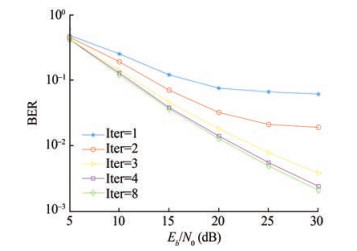Figure  8  Change in data symbol detection error with SNR under iterative verification

Download: Full-Size Img

Figure 9 shows the effect of data detection error on channel estimation accuracy. The symbol detection error refers to the average error of the data symbols in the range of n ∈ {n^′ − 4, ⋯, n^′ + 4} because only the data symbols in this range have an impact on the channel estimation at time n. The curves in Figure 9 are the results of eight iterative verifications. The three CEs in Figure 9 are based on the proposed data reuse method in this paper. Therefore, the performance of the three CEs is affected by symbol detection error. The estimation error of the three CEs generally increases with the data symbol detection error rate. The SBL-based CE shows the best performance, and the performance of the three CEs is relatively close.

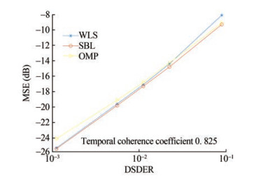Figure  9  Influence of data detection error on channel estimation accuracy

Download: Full-Size Img

4.2   Experiment results

The sea trial was conducted at sea near Zhoushan Archipelago, China, on December 6, 2022. Figure 10 shows the configuration and sound speed profile of the sea trial. The average water depth of the experimental sea area is approximately 40 m, the transceivers were placed beneath the water surface approximately 10 m, and the distance between the transmitter and the receiver is approximately 1 000 m.

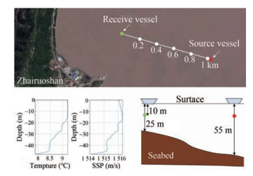Figure  10  Configuration of the sea trial

Download: Full-Size Img

The frame structure of the transmitted signal is shown in Figure 11, where the hyperbolic frequency modulation pulse is used for signal synchronization and Doppler estimation. 511-order m-sequence (M-seq) is used for fine synchronization and carrier frequency offset (CFO) estimation. The modulation parameters of the signal block, namely the average SNR of the signal received, is 21.5 dB. The parameters of signal block "FBMC 2" are consistent with the simulation in Section 4.1; that is, M = 128 and N = 30. The bandwidth is 3 000 Hz, and the center frequency f_c = 15 kHz. The number of the signal block subcarriers "FBMC 1" is 256, and other modulation parameters are the same as "FBMC 2."

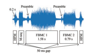Figure  11  Frame structure of sea trial transmission signal. The upper part is an actual sea trial receiving waveform with SNR=21.5 dB

Download: Full-Size Img

The source and receiver vessels slowly drifted with the current during the experiment. The estimated average CFO is 3.4 Hz. Channel estimation is performed on the received signal after frequency offset compensation, and the results are shown in Figure 12. Figure 12(a) shows the estimated modulus of the time-varying CIR. Results showed that the actual sea trial channels are similar to the computer simulation results. That is, the index of the main non-zero taps in the channels almost remains unchanged within an FBMC signal block period, but their amplitudes change. Figure 12(b) shows the time-varying phase of the main non-zero taps. The bold solid line is the phase change of the direct path. In addition to the direct path, the main non-zero taps can be divided into two groups. The taps of "group 2" correspond to the paths which reflect more times at the sea surface and bottom than the taps of "group 1." The taps of "group 2" are affected by more time-varying factors than "group 1" due to the long propagation time and additional reflection times in the channel, resulting in strong time-varying amplitude and phase. The four dotted lines in Figure 12(b) represent the phase changes of the four non-zero taps in group 2, and the four solid lines are the phase changes of the non-zero taps in group 1. Each phase curve continuously and slowly changes without mutations, indicating a strong correlation between channels at adjacent times.

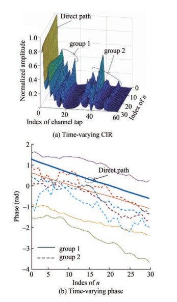Figure  12  Estimated time-varying channels of the sea trial

Download: Full-Size Img

Figure 13 shows the temporal coherence function of the sea trial channel to further describe the correlation between channels quantitatively. The blue solid line corresponds to the long signal block named "FBMC 1, " and the orange solid line with a circle mark corresponds to the short signal block named "FBMC 2." The declining slope of the orange curve is lower than that of the blue curve. The value of parameter N in the two signal blocks is the same. However, the correlation between channels in signal block "FBMC 2" is strong due to its short signal period.

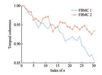Figure  13  Time coherence function of sea trial channel

Download: Full-Size Img

Figure 14 displays the demodulation results of block "FBMC 1" and block "FBMC 2" using a time-invariant channel (TIC) and time-varying channel (TVC), respectively. If the TICs were used, then the demodulation results of the long FBMC-OQAM symbol block would become worse with the increase of n. However, if the TVCs were tracked, then the BER does not increase with the n. In addition, the BER is low when M is small because the symbol period shortens with the decrease in M, and the short symbol period indicates a weak influence of TVC. For the FBMC-OQAM signal with a received SNR of approximately 21.5 dB, the average BER of symbol block "FBMC 1" generally decreases by 25.5 dB, and the average BER of symbol block "FBMC 2" decreases by 28.8 dB when using the proposed TVC tracking method.

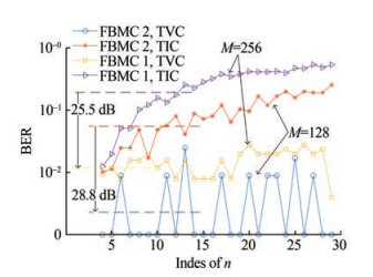Figure  14  Sea trial data demodulation results of the proposed CE with WLS criterion

Download: Full-Size Img

Table 2 and Figure 15 show the demodulation results of sea trial data with different channel tracking methods. These results show that the BER of short data block "FBMC 2" is low because the short data packets are only slightly affected by the TVC and the highly accurate channel tracking. However, the data block cannot be excessively short in practical applications. Ensuring that one FBMC multicarrier symbol is generally substantially longer than the channel delay is necessary; otherwise, insufficient alternatives will emerge when selecting new pilots. This phenomenon will lead to poor iterative verification effect on improving channel tracking accuracy.

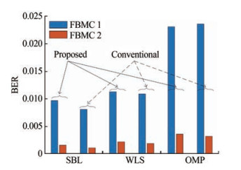Figure  15  Proposed low-overhead CE shows a performance close to that of the conventional high-overhead CE

Download: Full-Size Img

Considering system overhead, the proposed estimator based on data reuse in this paper has the minimum overhead and ensures the maximum data rate. For conventional channel estimation methods based on known pilots, the number of pilots for WLS-, OMP-, and SBL-based CEs is 64, 32, and 64, respectively.

5   Conclusions

A low-overhead channel tracking algorithm is proposed in this paper for short-range high-rate UWA FBMC-OQAM communication applications. By extending the UTM model to TVCs, the UTM symbol detector can approximately detect all interference symbols that are under the influence of TVC; then, utilize estimated interference symbols to eliminate interference for the selected new pilots. Multiple iterative verifications can improve the accuracy of channel tracking and data detection. The simulation results show that the channel tracking error can be reduced to less than −20 dB when the channel temporal coherence coefficient exceeds 0.75 within one block period of FBMC-OQAM signals. The proposed method shows that compared with conventional known-pilots-based methods, our method requires lower overhead without reducing the CE performance. The sea trial results further proved the practicability of the proposed method under the actual UWA communication scenarios.