Autopilot Design for an Unmanned Surface Vehicle Based on Backstepping Integral Technique with Experimental Results
https://doi.org/10.1007/s11804-023-00356-4
-
Abstract
Controller tuning is the correct setting of controller parameters to control complex dynamic systems appropriately and with high accuracy. Therefore, this study addressed the development of a method for tuning the heading controller of an unmanned surface vehicle (USV) based on the backstepping integral technique to enhance the vehicle behavior while tracking a desired position for water monitoring missions. The vehicle self-steering system (autopilot system) is designed theoretically and tested via a simulation. Based on the Lyapunov theory, the stability in the closed-loop system is guaranteed, and the convergence of the heading tracking errors is obtained. In addition, the designed control law is implemented via a microcontroller and tested experimentally in real time. Conclusion, experimental results were carried out to verify the robustness of the designed controller when disturbances and uncertainties are introduced into the system.Article Highlights● Nonlinear heading controller design using backstepping integral technique.● Controller tuning.● Autopilot system design for self-steering an Unmanned Surface Vehicle for waypoint tracking. -
1 Introduction
In the past decade, physicists have developed several mathematical models for studying wind (Bazionis and Georgilakis, 2021; Feijóo and Villanueva, 2016) and wave (Jeng et al., 2013) dynamics that have a considerable impact on the dynamics of sailing boats (Abrougui and Nejim, 2018).
Although environmental-force models are still insufficient to simulate the real behavior of the marine environment, these models can help researchers to understand and analyze the behavior of vessels and to design autopilot systems. Hence, Fossen made an assumption using the superposition of wind and wave disturbances (Fossen, 2011). Within the same framework, the authors of a previous study (Hu and Juang, 2011) designed a robust nonlinear course-keeping control method to control an unmanned surface vehicle (USV) under the influence of high wind forces and large wave disturbances.
Generally, the effects of disturbing elements such as wind and waves must be considered when designing autopilot systems. The latter requires either data from many sensors, such as wind vanes, anemometers, and speedometers, or the estimation of some parameters, such as ocean current speed and direction, to enhance tracking accuracy.
The proportional integral derivative (PID) control technique (Caccia et al., 2008; Song et al., 2022; Park et al., 2010; Qi et al., 2007) represents the first implemented control algorithm in autopilot system designs. Most self-steering systems were designed using PID control method (Wang and Ackermann, 1998). Several course-keeping control techniques have also been presented in previous studies, including the fuzzy control technique (Hearn et al., 1997), adaptive control based on gain scheduling (Liu et al., 2017), neural network method (Ma et al., 2019), model predictive control (Siramdasu and Fahimi, 2012; Sharma et al., 2013; Bai et al., 2022), intelligent control using the genetic algorithm (Zhang et al., 2019), local control network approach (Sharma et al., 2012) and linear quadratic Gaussian control method (Asfihani et al., 2019).
Advanced control approaches, such as feedback linearization techniques (Phanthong et al., 2014; Winursito et al., 2022) and sliding mode control (Abrougui et al., 2021; Chen et al., 2019; Ashrafiuon et al., 2008; Gonzalez-Garcia and Castañeda, 2021), were designed to improve the system robustness with respect to modeling uncertainties.
In this study, we propose the design of an autopilot system based on the backstepping integral technique used for waypoint tracking control. The heading controller was designed on the basis of external forces generated by ocean currents. The autopilot system demonstrated good performance during waypoint tracking in simulation and sea trials.
The remainder of this paper is structured as follows: The development of the mathematical model of the considered vehicle is presented in the second section. The heading controller, based on the backstepping integral method, is presented in the third section. The main contribution of this work is the tune of the developed heading controller.
The last section of this study addresses the design of a microcontroller-based autopilot system. Experimental results were presented to validate the developed control approach.
2 System modeling
2.1 Reference systems and vehicle description
The considered USV is presented in Figures 1 and 2. Figure 3 shows that the inertial reference frame R0 is (O, X0, Y0, Z0) and the body fixed frame R is (G, X, Y, Z). The origin of the body frame R is assumed to coincide with the USV's center of gravity as shown in Figure 3.
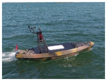 Figure 1 Unmanned surface vehicle used herein
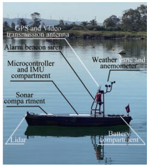 Figure 2 Hardware architecture of the USV
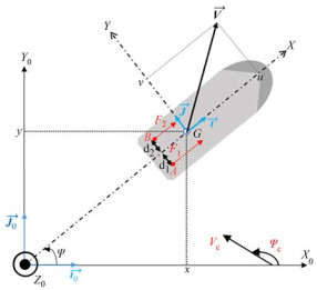 Figure 3 USV and reference systems
The USV actuator is composed of four electric motors, as illustrated in Figure 4.
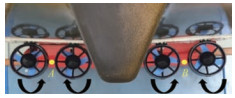 Figure 4 Rear view of thrusters
Thrusters control the USV heading and speed simultaneously by generating propulsion forces F1 and F2 on points A and B, respectively.
2.2 Equations of motion
The mathematical model of the USV can be simplified by using the following assumptions:
- Only surge u, sway v, and yaw r motions are modeled.
- The added-mass coefficients are modeled as constants.
All the variables used herein are presented and described in Table 1.
Table 1 Variable descriptionNotation Description u Surge velocity v Sway velocity r Yaw rate ψ Heading angle F2 Left thrust force applied in A F1 Right thrust force applied in B m USV mass Iz Inertial moment around the GZ axis x, y USV position in the R0 frame ψc Direction of the marine current Vc Speed of the marine current $X_{\dot{u}}, Y_{\dot{v}}$ Added mass along the GX, GY axes $N_{\dot{r}}$ Added mass around the GZ axes d = d1 = d2 Distance between A and B horizontally J (η) Transformation matrix from the R-frame to the fixed frame Therefore, the USV velocity expressed in the body frame is expressed as ϑ = [u v r]T.
Let us define η = [x y ψ]T. This parameter describes the USV position (x, y) and heading ψ in the inertial frame.
On the basis of Fossen's model (Fossen, 2011), the USV mathematical model (vectorial form) can be presented as follows:
$$ \dot{\eta}=J(\eta) \vartheta $$ (1) $$ \boldsymbol{M}_{\mathrm{RB}} \dot{\vartheta}+\boldsymbol{M}_A \dot{\vartheta}_r+\boldsymbol{C}_{\mathrm{RB}} \vartheta+\boldsymbol{C}_A \vartheta_r+\boldsymbol{D}=\tau_1+\tau_2 $$ (2) with
$$ \boldsymbol{J}(\eta)=\left[\begin{array}{ccc} \cos \psi & -\sin \psi & 0 \\ \sin \psi & \cos \psi & 0 \\ 0 & 0 & 1 \end{array}\right] $$ (3) MRB and MA are the rigid and added-mass matrices, respectively.
$$ \boldsymbol{M}_{\mathrm{RB}}=\left[\begin{array}{ccc} m & 0 & 0 \\ 0 & m & 0 \\ 0 & 0 & I_z \end{array}\right] $$ (4) $$ \boldsymbol{M}_A=-\left[\begin{array}{ccc} X_{\dot{u}} & 0 & 0 \\ 0 & Y_{\dot{v}} & 0 \\ 0 & 0 & N_{\dot{r}} \end{array}\right] $$ (5) ϑr = (ur vr r)T is the boat velocity relative to the water, which is expressed as follows:
$$ \left[\begin{array}{l} u_r \\ v_r \end{array}\right]=\left[\begin{array}{l} u \\ v \end{array}\right]-\left[\begin{array}{cc} \cos \psi & \sin \psi \\ -\sin \psi & \cos \psi \end{array}\right]\left[\begin{array}{c} V_C \cos \psi_C \\ V_C \sin \psi_C \end{array}\right] $$ (6) CRB and CA are the rigid-body Coriolis-centripetal and added-mass Coriolis matrices, respectively.
$$ \boldsymbol{C}_{\mathrm{RB}}=\left[\begin{array}{ccc} 0 & -m r & 0 \\ m r & 0 & 0 \\ 0 & 0 & 0 \end{array}\right] $$ (7) $$ \boldsymbol{C}_A=\left[\begin{array}{ccc} 0 & 0 & Y_{\dot{v}} v_r \\ 0 & 0 & -X_{\dot{u}} u_r \\ -Y_{\dot{v}} v_r & X_{\dot{u}} u_r & 0 \end{array}\right] $$ (8) $$ \boldsymbol{D}=\left[\begin{array}{ccc} g_1\left(u_r\right) & 0 & 0 \\ 0 & g_2\left(v_r\right) & 0 \\ 0 & 0 & g_3(r) \end{array}\right] $$ (9) where g1(ur) = α1urβ1: surge resistance model along the GX axis; g2(vr) = α2vrβ2: sway resistance model along the GY axis; g3(r) = α3rβ3: yaw resistance model around the GZ axis; τ1 and τ2 are respectively the thrust force and the yaw moment. They are given as follows:
$$ \tau_1=\left[\begin{array}{c} F_1+F_2 \\ 0 \\ 0 \end{array}\right] $$ (10) $$ \tau_2=\left[\begin{array}{c} 0 \\ 0 \\ \left(F_2-F_1\right) d \end{array}\right] $$ (11) By using property 8.1 in (Fossen, 2011),
$$ \boldsymbol{M}_{\mathrm{RB}} \dot{\vartheta}+\boldsymbol{C}_{\mathrm{RB}} \vartheta=\boldsymbol{M}_{\mathrm{RB}} \dot{\vartheta}_r+\boldsymbol{C}_{\mathrm{RB}} \vartheta_r $$ (12) Equation (2) becomes
$$ \left(m-X_{\dot{u}}\right) \dot{u}_r=\tau_1+r v_r\left(m+Y_{\dot{v}}\right)-g_1\left(u_r\right) $$ (13) $$ \left(m-Y_{\dot{v}}\right) \dot{v}_r=-r u_r\left(m+X_{\dot{u}}\right)-g_2\left(v_r\right) $$ (14) $$ \left(I_z-N_{\dot{r}}\right) \dot{r}=\tau_2-u_r v_r\left(Y_{\dot{v}}-X_{\dot{u}}\right)-g_3(r) $$ (15) Finally, a three degrees of freedom (3DOF) dynamic model of the USV is given as follows:
$$ \left\{\begin{array}{c} \dot{x}=u \cos \psi-v \sin \psi \\ \dot{y}=u \sin \psi+v \cos \psi \\ \dot{\psi}=r \\ \dot{u}_r=\frac{\tau_1+r v_r\left(m+Y_{\dot{v}}\right)-g_1\left(u_r\right)}{m-X_{\dot{u}}} \\ \dot{v}_r=\frac{-r u_r\left(m+X_{\dot{u}}\right)-g_2\left(v_r\right)}{m-Y_{\dot{v}}} \\ \dot{r}=\frac{\tau_2-\left(Y_{\dot{v}}-X_{\dot{u}}\right) u_r v_r-g_3(r)}{I_z-N_{\dot{r}}} \\ u=u_r+V_C \cos \left(\psi-\psi_C\right) \\ v=v_r-V_C \sin \left(\psi-\psi_C\right) \end{array}\right. $$ (16) The mathematical model (16) is highly nonlinear and has the form of $\dot{X}=f(\boldsymbol{X}, \boldsymbol{U})$, where X = (x y ψ ur vr r)T is the state vector, and U = (τ1τ2)T is the input control vector. Hydrodynamic coefficients were identified as described in a previous study (Abrougui et al., 2021). As discussed in the following section, a heading controller was designed and tested via simulation when the vehicle had to track desired waypoints.
3 Control system design
Theorem 1An autonomous system $\dot{x}=f(x)$ has an equilibrium point xe = 0, which is globally and asymptotically stable if a continuous scalar function V (x) with the following properties exists (Bacciotti and Rosier, 2005):
$$ \left\{\begin{array}{c} V(0)=0 \\ V(x)>0 \quad \forall x \neq 0 \\ \lim _{x \rightarrow+\infty} V(x)=+\infty \\ \dot{V}(x)<0 \quad \forall x \neq 0 \end{array}\right. $$ (17) Proof: Let us consider a system written in the following form:
$$ \left\{\begin{array}{c} \dot{x}_1=f_1\left(x_1\right)+g_1\left(x_1\right) x_2 \\ \dot{x}_2=f_2\left(x_1, x_2\right)+g_2\left(x_1, x_2\right) u(t) \end{array}\right. $$ (18) where f and g are nonlinear functions, and u(t) is the input control. u(t) should be calculated by allowing x1 to converge to a setpoint x1d.
First, let us define the error of the first variable x1 as
$$ e_1=x_{1 d}-x_1 $$ (19) Its time derivative is
$$ \dot{e}_1=\dot{x}_{1 d}-\dot{x}_1=\dot{x}_{1 d}-f_1\left(x_1\right)-g_1\left(x_1\right) x_2 $$ (20) Let us define the Lyapunov candidate function as follows:
$$ V_1=\frac{1}{2} e_1^2+\frac{\beta_1}{2} \sigma^2 $$ (21) with $\dot{\sigma}=e_1$, and β1 is a positive design parameter.
The time derivative of V1 is
$$ \begin{aligned} \dot{V}_1 & =e_1 \dot{e}_1+\beta_1 \sigma e_1 \\ & =e_1\left(\dot{x}_{1 d}-f_1\left(x_1\right)-g_1\left(x_1\right) x_2+\beta_1 \sigma\right) \end{aligned} $$ (22) The virtual control input x2 should be equal to x2d, as given in the following equation. Letting $\dot{V}(x)<0$:
$$ x_{2 d}=\frac{1}{g_1\left(x_1\right)}\left(k_1 e_1-f_1\left(x_1\right)+\dot{x}_{1 d}+\beta_1 \sigma\right) $$ (23) where k1 > 0 is a design parameter, and g1(x1) ≠ 0.
By substituting Equation (23) into (22), we obtain
$$ \dot{V}_1=-k_1 e_1^2 <0 $$ (24) Second, let us define the error of the second variable as
$$ e_2=x_{2 d}-x_2 $$ (25) The time derivative of e2 is given by
$$ \dot{e}_2=\dot{x}_{2 d}-\dot{x}_2=\dot{x}_{2 d}-f_2\left(x_1, x_2\right)-g_2\left(x_1, x_2\right) u(t) $$ (26) Let us define the Lyapunov candidate function as follows:
$$ V_2=V_1+\frac{1}{2} e_2^2 $$ (27) Its time derivative is given by
$$ \begin{aligned} \dot{V}_2 & =\dot{V}_1+e_2 \dot{e}_2 \\ & =e_1 \dot{e}_1+\beta_1 \sigma e_1+e_2\left(\dot{x}_{2 d}-f_2\left(x_1, x_2\right)-g_2\left(x_1, x_2\right) u(t)\right) \end{aligned} $$ (28) In the case of x2 ≠ x2d, we have,
$$ \begin{aligned} \dot{e}_1 & =\dot{x}_{1 d}-\dot{x}_1 \\ & =\dot{x}_{1 d}-f_1\left(x_1\right)-g_1\left(x_1\right) x_2 \\ & =\dot{x}_{1 d}-f_1\left(x_1\right)-g_1\left(x_1\right)\left(x_{2 d}-e_2\right) \\ & =\dot{x}_{1 d}-f_1\left(x_1\right)+g_1\left(x_1\right) e_2-k_1 e_1+f_1\left(x_1\right)-\dot{x}_{1 d}-\beta_1 \sigma \\ & =g_1\left(x_1\right) e_2-k_1 e_1-\beta_1 \sigma \end{aligned} $$ (29) Equation (28) becomes
$$ \begin{aligned} \dot{V}_2= & e_1\left[g_1\left(x_1\right) e_2-k_1 e_1-\beta_1 \sigma\right]+\beta_1 \sigma e_1 \\ & +e_2\left[\dot{x}_{2 d}-f_2\left(x_1, x_2\right)-g_2\left(x_1, x_2\right) u(t)\right] \\ = & g_1\left(x_1\right) e_2 e_1-k_1 e_1^2 \\ & +e_2\left[\dot{x}_{2 d}-f_2\left(x_1, x_2\right)-g_2\left(x_1, x_2\right) u(t)\right] \end{aligned} $$ (30) The input control u(t) should be expressed as follows to obtain $\dot{V}_2 <0$.
$$ u=\frac{1}{g_2\left(x_1, x_2\right)}\left(k_2 e_2-f_2\left(x_1, x_2\right)+\dot{x}_{2 d}+g_1\left(x_1\right) e_1\right) $$ (31) where k2 > 0 is a design parameter, and g2(x1, x2) ≠ 0. Let pose g1(x1) = g1. The time derivative of Equation (23) is given by
$$ \dot{x}_{2 d}=\frac{1}{g_1}\left(k_1 \dot{e}_1-\dot{f}_1\left(x_1\right)+\ddot{x}_{1 d}+\beta_1 e_1\right) $$ (32) By substituting Equation (32) into (30), we obtain
$$ \dot{V}_2=-k_1 e_1^2-k_2 e_2^2 <0 $$ (33) Hence, the Lyapunov candidate function (27) decreases gradually, indicating that (e1, $\dot{e}_1$) converge to 0 as t → +∞. Therefore, stability in the closed-loop system is established.
3.1 Heading controller design
From (16), we can extract the USV yaw dynamics as follows:
$$ \left\{\begin{array}{c} \dot{\psi}=r \\ \dot{r}=\frac{\tau_2-\left(Y_{\dot{v}}-X_{\dot{u}}\right) u_r v_r-g_3(r)}{I_z-N_{\dot{r}}} \end{array}\right. $$ (34) First, let us define the heading error e1 as e1 = ψd − ψ. Its time derivative is
$$ \dot{e}_1=\dot{\psi}_d-r $$ (35) Let us define the following Lyapunov candidate function as
$$ V_1=\frac{1}{2} e_1^2+\frac{\beta}{2} \sigma^2 $$ (36) with $\dot{\sigma}=e_1$.
The time derivative of V1 is
$$ \dot{V}_1=e_1 \dot{e}_1+\beta \sigma e_1=e_1\left(\beta \sigma+\dot{\psi}_d-r\right) $$ (37) From Equation (37), variable r should converge to rd to ensure $\dot{V}_1 <0$.
$$ r_d=k_1 e_1+\beta \sigma+\dot{\psi}_d $$ (38) Using Equations (37) and (38), we obtain
$$ \dot{V}_1=-k_1 e_1^2 <0 $$ (39) where k1 > 0 is a design control parameter.
Second, let us define the error e2 of the variable r as
$$ e_2=r_d-r $$ (40) Its time derivative is expressed as
$$ \dot{e}_2=\dot{r}_d-\dot{r} $$ (41) Let us define the following Lyapunov candidate function as follows:
$$ V_2=V_1+\frac{1}{2} e_2^2 $$ (42) Its time derivative is given by
$$ \begin{aligned} \dot{V}_2 & =\dot{V}_1+e_2 \dot{e}_2 \\ & =e_1 \dot{e}_1+\beta \sigma e_1+e_2 \dot{e}_2 \\ & =e_1\left(\dot{\psi}_d-r\right)+\beta \sigma e_1+e_2 \dot{e}_2 \\ & =e_1\left(\dot{\psi}_d-\left(r_d-e_2\right)\right)+\beta \sigma e_1+e_2\left(\dot{r}_d-\dot{r}\right) \end{aligned} $$ (43) where $r_d=k_1 e_1+\beta \sigma+\dot{\psi}_d$. Therefore, we obtain
$$ \dot{V}_2=e_1\left(e_2-k_1 e_1\right)+e_2\left(\dot{r}_d-\dot{r}\right) $$ (44) The angular acceleration ṙ is chosen as follows to verify $\dot{V}_2 <0$:
$$ \dot{r}=k_2 e_2+e_1+\dot{r}_d $$ (45) where k2 > 0 is a design control parameter and
$$ \dot{r}_d=k_1 \dot{e}_1+\beta e_1+\ddot{\psi}_d $$ (46) Using (44) and (45), we acquire
$$ \dot{V}_2=-k_1 e_1^2-k_2 e_2^2 <0 \quad \forall\left(e_1, e_2\right) \neq(0, 0) $$ (47) Therefore, using (34) and (45), the heading controller τ2 is expressed as follows:
$$ \begin{aligned} \tau_2= & \left(I_z-N_{\dot{r}}\right)\left(k_2 e_2+e_1+\dot{r}_d\right)+\left(Y_{\dot{v}}-X_{\dot{u}}\right) u_r v_r+g_3(r) \\ = & \left(I_z-N_{\dot{r}}\right)\left(e_1\left(1+\beta+k_1 k_2\right)-r\left(k_2+k_1\right)-\beta \sigma k_2\right)+ \\ & \left(Y_{\dot{v}}-X_{\dot{u}}\right) u_r v_r+g_3(r) \end{aligned} $$ (48) with
$$ \begin{aligned} & u_r=u-V_C \cos \left(\psi-\psi_C\right) \\ & v_r=v+V_C \sin \left(\psi-\psi_C\right) \end{aligned} $$ The parameters k1, k2, and β that remain to be determined are as follows:
From Equation (38), we have
$$ \dot{\psi}_d=r_d-k_1 e_1-\beta \sigma $$ (49) Therefore, Equation (35) becomes
$$ \begin{aligned} \dot{e}_1 & =\dot{\psi}_d-r \\ & =r_d-k_1 e_1-\beta \sigma-r \\ & =\left(r_d-r\right)-k_1 e_1-\beta \sigma \\ & =e_2-k_1 e_1-\beta \sigma \end{aligned} $$ (50) Using Equations (41) and (45), we obtain
$$ \dot{e}_2=-k_2 e_2-e_1 $$ (51) Consequently, we have
$$ \left\{\begin{array}{c} \dot{e}_1=e_2-k_1 e_1-\beta \sigma \\ \dot{e}_2=-k_2 e_2-e_1 \\ \dot{\sigma}=e_1 \end{array}\right. $$ (52) Therefore, we have
$$ \left[\begin{array}{c} \dot{e}_1 \\ \dot{e}_2 \\ \dot{\sigma} \end{array}\right]=\left[\begin{array}{ccc} -k_1 & 1 & -\beta \\ -1 & -k_2 & 0 \\ 1 & 0 & 0 \end{array}\right]\left[\begin{array}{c} e_1 \\ e_2 \\ \sigma \end{array}\right] $$ (53) The characteristic polynomial is
$$ \begin{aligned} P(s) & =\left|\begin{array}{ccc} s+k_1 & -1 & \beta \\ 1 & s+k_2 & 0 \\ -1 & 0 & s \end{array}\right| \\ & =s^3+\left(k_1+k_2\right) s^2+\left(k_1 k_2+\beta+1\right) s+k_2 \beta \end{aligned} $$ (54) It has the following form:
$$ P(s)=\left(s-s_0\right)\left(s-s_1\right)\left(s-s_2\right) $$ (55) where s0, s1, s2 are designed as three poles allowing the heading dynamic to behave as desired.
(s − s1) (s − s2) can be seen as a second-order polynomial with s1 = s2. It can be written in the form of s2 + 2ξωs + ω2, where ξ = 1 is the damping ratio, and ω is the undamped natural frequency.
If we want to force the third-order system (55) to behave like a second-order system, we have to choose |s0| ≫ |s1| as ξ = 1. According to Figure 5, $\omega=\frac{5}{t_{r 5 \%}}$, where tr 5% is the desired 5% response time.
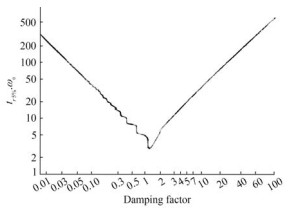 Figure 5 Response time of the second-order system as function of the damping ratio
Let us select |s0| = 20|s1| to obtain |s0| ≫ |s1|. By developing the polynomial (s + 20ω) (s + ω)2 and using (55), we obtain
$$ \left\{\begin{array}{c} k_1+k_2=22 \omega \\ k_1 k_2+\beta+1=41 \omega^2 \\ k_2 \beta=20 \omega^3 \end{array}\right. $$ (56) By choosing tr 5% = 3s, we obtain k1 = 3.3 and k2 = 33.37 at β = 2.775.
3.2 High-level controller design
Guidance is a system that generates the desired heading ψd to be used as input into the heading controller (Figure 6).
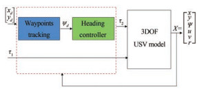 Figure 6 Autopilot scheme
The desired heading ψd can be given by
$$ \psi_d=\tan ^{-1}\left(\frac{y-y_d}{x-x_d}\right) $$ (57) (x, y) is the actual position of the USV, and (xd, yd) the desired position of the USV. ψd represents the direction to the target position (line of sight).
τ1 is chosen constant and equal to 50% of the total thrust force during the simulation and experimental tests.
4 Simulation and experimental results
4.1 Simulation results
A simulation test was conducted to test the performance of the proposed method for tuning the heading controller. In this context, we introduced three target positions into the guidance system.
The ocean current velocity and direction were set to (Vc = 0.1 m/s, ψc = − 90°), and the used normalized parameters (Abrougui et al., 2021) are given in Table 2.
Table 2 Evaluation of ParametersNotation Value $X_{\dot{u}}(\mathrm{~kg} / \mathrm{N})$ 4.5×10⁻⁴ $Y_{\dot{v}}(\mathrm{~kg} / \mathrm{N})$ 1.8×10⁻³ $N_{\dot{r}}\left(\mathrm{~kg} \cdot \mathrm{m}^2 / \mathrm{N}\right)$ 2.16×10⁻² m (kg/N) 0.009 Iz(kg·m2/N) 6×10⁻² d (m) 0.24 α1 0.329 9 β1 1.646 6 α2 4 β2 1 α0 0.24 α3 0.85 β3 1 The path of the USV is shown in Figure 7. The desired waypoints were well reached by the USV despite the presence of model uncertainties and disturbances owing to the ocean current
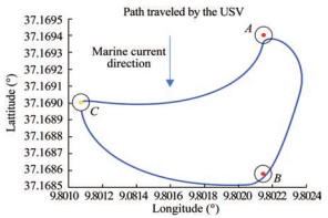 Figure 7 Path followed by the USV during the simulation
The time evolution of the USV heading, as illustrated in Figure 8, shows that the system responded rapidly, accurately, and without overshooting during the steady state as desired.
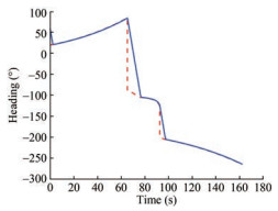 Figure 8 Time evolution of the USV heading
Figure 9 presents the evolution of the yaw rate. The yaw rate was constantly equal to zero unless the USV heading changed.
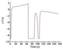 Figure 9 Yaw rate
Figure 10 shows that the heading error is always zero as demonstrated in section 3. Consequently, the effectiveness of the proposed method in terms of the accuracy of the designed controller was proven.
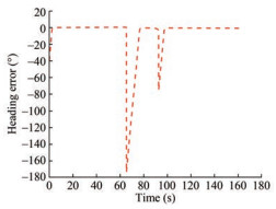 Figure 10 Time evolution of the heading error e1 (t)
The controller τ2 (Figure 11) is capable of providing control action to minimize the error in heading. Figure 12 shows also that the generated control inputs for left and right thrusts were smooth. Moreover, no chattering problem was observed. These satisfactory tracking performances clearly demonstrate the efficiency of the heading controller tuning approach.
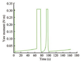 Figure 11 Yaw moment
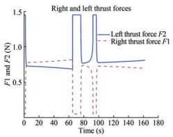 Figure 12 Yaw moment
4.2 Experimental results
As discussed in this section, an ATMega2560 microcontroller was used to implement the developed autopilot approach (see the hardware architecture of the autopilot system described in Figure 13). The designed heading controller (Equation (48)) was implemented via the Arduino integrated development environment. The parameters k1, k2, and β were calculated as described in Section 3.1.
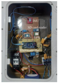 Figure 13 Proposed autopilot system hardware
Figure 12 presents the system hardware, which comprises
• an inertial measurement unit (MPU 9250 with its library from GitHub),
• a GPS (NEO 7M) for measuring the USV position and speed on the ground;
• a SD card reader for data logging.
As shown in Figures 14 and 15, the USV reached all the waypoints 1, 2, and 3, even in the presence of environmental disturbances due to ocean currents.
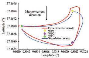 Figure 14 Paths followed by the USV during the simulation and experimental tests
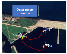 Figure 15 Path followed by the USV during the experimental test
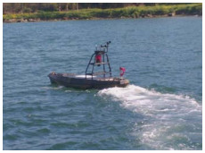 Figure 16 USV whenreaching waypoints
In contrast to the simulation result presented in Figure 9, the experimental results in Figures 17 and 18 illustrate that the USV heading converged to the desired heading with some fluctuations, which occurred owing to the noisy measurements originating from the compass sensor.
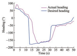 Figure 17 Time evolution of the desired and actual heading during the experimental test (sample time is 35 ms)
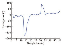 Figure 18 Time evolution of the heading error during the experimental test (sample time is 35 ms)
Figure 19 shows the time evolution of the designed controller τ2 (yaw moment) during the experimental test letting the USV heading to track desired ones in order to reach all the given waypoints successively. The calculated yaw moment was converted into a pulse-width modulation PWM signal for controlling the differential thrust force via a microcontroller.
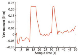 Figure 19 Time evolution of the input control during the experimental test (sample time is 35 ms)
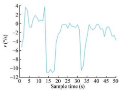 Figure 20 Time evolution of the yaw rate during the experimental test (sample time is 35 ms)
5 Conclusions
This study addressed the design of an autopilot system for controlling a USV. In a previous study (Abrougui et al., 2021), the sliding mode control was applied, evaluated, and tested in real time for controlling the USV. In this study, another technique was used to develop an autopilot system based on the backstepping integral method. The control stability of the developed system was proven based on Lyapunov theory. An approach for tuning the heading controller was also proposed and tested. Simulation and experimental results were presented to demonstrate the effectiveness of the proposed control law. The next work will be conducted to add an obstacle avoidance system to the proposed autopilot.
Acknowledgement: The authors would like to thank the Ministry of Defense and the Tunisian Naval Academy for supporting this work.Competing interest The authors have no competing interests to declare that are relevant to the content of this article. -
Figure 1 Unmanned surface vehicle used herein
Figure 2 Hardware architecture of the USV
Figure 3 USV and reference systems
Figure 4 Rear view of thrusters
Figure 5 Response time of the second-order system as function of the damping ratio
Figure 6 Autopilot scheme
Figure 7 Path followed by the USV during the simulation
Figure 8 Time evolution of the USV heading
Figure 9 Yaw rate
Figure 10 Time evolution of the heading error e1 (t)
Figure 11 Yaw moment
Figure 12 Yaw moment
Figure 13 Proposed autopilot system hardware
Figure 14 Paths followed by the USV during the simulation and experimental tests
Figure 15 Path followed by the USV during the experimental test
Figure 16 USV whenreaching waypoints
Figure 17 Time evolution of the desired and actual heading during the experimental test (sample time is 35 ms)
Figure 18 Time evolution of the heading error during the experimental test (sample time is 35 ms)
Figure 19 Time evolution of the input control during the experimental test (sample time is 35 ms)
Figure 20 Time evolution of the yaw rate during the experimental test (sample time is 35 ms)
Table 1 Variable description
Notation Description u Surge velocity v Sway velocity r Yaw rate ψ Heading angle F2 Left thrust force applied in A F1 Right thrust force applied in B m USV mass Iz Inertial moment around the GZ axis x, y USV position in the R0 frame ψc Direction of the marine current Vc Speed of the marine current $X_{\dot{u}}, Y_{\dot{v}}$ Added mass along the GX, GY axes $N_{\dot{r}}$ Added mass around the GZ axes d = d1 = d2 Distance between A and B horizontally J (η) Transformation matrix from the R-frame to the fixed frame Table 2 Evaluation of Parameters
Notation Value $X_{\dot{u}}(\mathrm{~kg} / \mathrm{N})$ 4.5×10⁻⁴ $Y_{\dot{v}}(\mathrm{~kg} / \mathrm{N})$ 1.8×10⁻³ $N_{\dot{r}}\left(\mathrm{~kg} \cdot \mathrm{m}^2 / \mathrm{N}\right)$ 2.16×10⁻² m (kg/N) 0.009 Iz(kg·m2/N) 6×10⁻² d (m) 0.24 α1 0.329 9 β1 1.646 6 α2 4 β2 1 α0 0.24 α3 0.85 β3 1 -
Abrougui H, Nejim S (2018) Backstepping control of an autonomous catamaran sailboat. Robotic Sailing, 41–50 Abrougui H, Nejim S, Hachicha S, Zaoui C, Dallagi H (2021) Modeling, parameter identification, guidance and control of an unmanned surface vehicle with experimental results. Ocean Engineering, 241, 110038 https://doi.org/10.1016/j.oceaneng.2021.110038 Asfihani T, Arif DK, Putra FP, Firmansyah MA (2019) Comparison of LQG and adaptive PID Controller for USV heading control. Journal of Physics: Conference Series 1218(1): 012058 https://doi.org/10.1088/1742-6596/1218/1/012058 Ashrafiuon H, Muske KR, McNinch LC, Soltan RA (2008) Slidingmode tracking control of surface vessels. IEEE Transactions on Industrial Electronics 55(11): 4004–4012 https://doi.org/10.1109/TIE.2008.2005933 Bacciotti A, Rosier L (2005) Lyapunov functions and stability in control theory. Springer Science & Business Media Bai X, Li B, Xu X, Xiao Y (2022) A review of current research and advances in unmanned surface vehicles. Journal of Marine Science and Application 21(2): 47–58 https://doi.org/10.1007/s11804-022-00276-9 Bazionis IK, Georgilakis PS (2021) Review of deterministic and probabilistic wind power forecasting: Models, methods, and future research. Electricity 2(1): 13–47 https://doi.org/10.3390/electricity2010002 Caccia M, Bibuli M, Bono R, Bruzzone G (2008) Basic navigation, guidance and control of an unmanned surface vehicle. Autonomous Robots 25(4): 349–365 https://doi.org/10.1007/s10514-008-9100-0 Chen Z, Zhang Y, Zhang Y, Nie Y, Tang J, Zhu S (2019) Disturbance-observer-based sliding mode control design for nonlinear unmanned surface vessel with uncertainties. IEEE Access 7: 148522–148530 https://doi.org/10.1109/ACCESS.2019.2941364 Feijóo A, Villanueva D (2016) Assessing wind speed simulation methods. Renewable and Sustainable Energy Reviews 56: 473–483 https://doi.org/10.1016/j.rser.2015.11.094 Fossen TI (2011) Handbook of marine craft hydrodynamics and motion control. John Wiley & Sons Gonzalez-Garcia A, Castañeda H (2021) Guidance and control based on adaptive sliding mode strategy for a USV subject to uncertainties. IEEE Journal of Oceanic Engineering 46(4): 1144–1154 https://doi.org/10.1109/JOE.2021.3059210 Hearn GE, Zhang Y, Sen P (1997) Alternative designs of neural network-based autopilots: a comparative study. IFAC Proceedings Volumes 30(22): 83–88 https://doi.org/10.1016/S1474-6670%2817%2946494-9 Hu SS, Juang JY (2011) Robust nonlinear ship course-keeping control under the influence of high wind and large wave disturbances. 8th Asian Control Conference, 393–398 Jeng DS, Ye JH, Zhang JS, Liu PF (2013) An integrated model for the wave-induced seabed response around marine structures: Model verifications and applications. Coastal Engineering 72: 1–19 https://doi.org/10.1016/j.coastaleng.2012.08.006 Liu L, Wang D, Peng Z, Li T (2017) Modular adaptive control for LOS-based cooperative path maneuvering of multiple underactuated autonomous surface vehicles. IEEE Transactions on Systems, Man, and Cybernetics: Systems 47(7): 1613–1624 https://doi.org/10.1109/TSMC.2017.2650219 Ma LY, Xie W, Huang HB (2019) Convolutional neural network-based obstacle detection for unmanned surface vehicle. Mathematical Biosciences and Engineering 17(1): 845–861 https://doi.org/10.3934/mbe.2020045 Park JH, Shim HW, Jun BH, Kim SM, Lee PM, Lim YK (2010) A model estimation and multi-variable control of an unmanned surface vehicle with two fixed thrusters. Oceans'10, Sydney, 1–5 Phanthong T, Maki T, Ura T, Sakamaki T, Aiyarak P (2014) Application of A* algorithm for real-time path re-planning of an unmanned surface vehicle avoiding underwater obstacles. Journal of Marine Science and Application 13(1): 105–116 https://doi.org/10.1007/s11804-014-1224-3 Qi J, Peng Y, Wang H, Han J (2007) Design and implement of a trimaran unmanned surface vehicle system. 2007 International Conference on Information Acquisition, 361–365 Sharma SK, Naeem W, Sutton R (2012) An autopilot based on a local control network design for an unmanned surface vehicle. J. Navigation 65(2): 281–301. DOI: https://doi.org/ 10.1017/S0373463311000701 Sharma SK, Sutton R, Motwani A, Annamalai A (2013) Non-linear control algorithms for an unmanned surface vehicle. Proceedings of the Institution of Mechanical Engineers, Part M, Journal of Engineering for the Maritime Environment 227(4): 1–10 Siramdasu Y, Fahimi F (2012) Incorporating input saturation for underactuated surface vessel trajectory tracking control. American Control Conference, Montreal, 6203–6208 Song L, Xu C, Hao L, Yao J, Guo R (2022) Research on PID parameter tuning and optimization based on SAC-Auto for USV path following. Journal of Marine Science and Engineering 10(12): 1847 https://doi.org/10.3390/jmse10121847 Wang L, Ackermann J (1998) Robustly stabilizing PID controllers for car steering systems. Proceedings of the 1998 American Control Conference, Philadelphia, 1, 41–42. DOI: https://doi.org/10.1109/ACC.1998.694624 Winursito A, Dhewa OA, Nasuha A, Pratama GN (2022) Integral state feedback controller with coefficient diagram method for USV heading control. 5th International Conference on Information and Communications Technology, 295–300 Zhang W, Xu Y, Xie J (2019) Path planning of USV based on improved hybrid genetic algorithm. European Navigation Conference, Warsaw, 1–7. DOI: https://doi.org/10.1109/EURONAV.2019.8714160