1   Introduction

Water transport plays an important role in economic developments and accounts for about 95% of global transportation tasks (Gu et al., 2023; Zereik et al., 2018; Wu et al., 2020; Campbell et al., 2012; Peng et al., 2021; Lv et al., 2022; Zhang et al., 2018; Wang et al., 2021). Unmanned surface vehicles (USVs) are versatile watercraft that can perform water transportation tasks with minimum human supervision (Li et al., 2022; Shi et al., 2017; Skjetne et al., 2005; Gu et al., 2021; Chen and Wei, 2014; Wu et al., 2021; Veremey, 2014; Wu et al., 2022a; Ma et al., 2018). Trajectory tracking and path following are two fundamental motion control problems for USVs (Qu et al., 2017; Aguiar and Hespanha, 2007; Paliotta et al., 2019; Jiang and Liang, 2018; Ma et al., 2022). In particular, trajectory tracking requires a USV to track a time-related trajectory (Peng et al., 2021; Yu et al., 2020; Katayama and Aoki, 2014; He et al., 2017; Li et al., 2018), whereas path following refers to forcing a USV to follow a path without strict temporal specifications. Path following takes an attractive decoupling property between the geometric task of controlling the USV position and the dynamic task of assigning a speed profile for virtual tracking (Wang et al., 2012; Meng et al., 2012; Deng et al., 2020; Abdurahman et al., 2019; Breivik et al., 2008; Wang et al., 2019; Fossen et al., 2017; Qu et al., 2017; Ma et al., 2021; Wu et al., 2022b; Peng et al., 2023).

In recent years, line-of-sight (LOS) guidance, as an intuitive and effective way to achieve path convergence, has been studied on the basis of path following. In Fossen and Pettersen (2014), a proportional LOS guidance law is proposed, and its uniform semi-global exponential stability is proven. In Caharijia et al. (2016), an integral LOS guidance law is constructed to compensate for the drift effect of environmental disturbances. In the study conducted by Belleter et al. (2019), an adaptive LOS guidance law is proposed to solve the problem of path following subject to constant ocean currents. In Liu et al. (2017), an extended state observer (ESO) -based LOS guidance law is proposed, where a reduced-order ESO is used to estimate the time-varying sideslip angle. Moreover, two ESOs are used to separately estimate surge and sway linear velocities (Yu et al., 2019a); that is, the unmeasured sideslip angle can be indirectly calculated and compensated on the basis of the LOS guidance law. In Yu et al. (2019b), a finite-time LOS-based guidance law is developed; that is, path following can be achieved within a finite time. However, the abovementioned LOS guidance methods only consider a USV running in an open-water area. With regard to a USV running in a constrained water region, e. g., inland rivers or canals, the abovementioned LOS guidance methods cannot be applied as safety cannot be ensured. In achieving path following in a constrained water region, an error-constrained LOS guidance law is proposed (Zheng et al., 2018; Zheng, 2020), where the path following tracking errors are constrained by using a tan-type barrier Lyapunov function method. Although the error-constrained LOS guidance method could avoid collisions with waterway boundaries by constraining tracking errors, it cannot address guidance moving in a constrained water region with multiple stationary and moving obstacles.

Given the abovementioned discussions, this paper investigates the safety-certificated LOS guidance of a USV in a constrained water region with multiple obstacles. First, an ESO is proposed to estimate unknown ocean currents. Next, a straight-line LOS guidance law is designed on the basis of the estimated information from the ESO. Then, in achieving a collision-free straight-line following task, control barrier functions (CBFs) are used to optimize the guidance signals where safe guidance signals are obtained by solving a quadratic programming problem. By using the proposed safe-certificated LOS guidance method, the USV can follow a straight-line path in a constrained water region while ensuring safety. Finally, the closed-loop guidance system can ensure input-to-state safety (ISSf) and that all error signals are uniformly and ultimately bounded. Simulation results are provided to substantiate the efficacy of the proposed safe-certificated LOS guidance method for straight-line following of a USV in a constrained water region.

• In contrast to the LOS guidance method proposed by Fossen and Pettersen (2014), Caharijia et al. (2016), Liu et al. (2016), Liu et al. (2017), Belleter et al. (2019), Yu et al. (2019a), Yu et al. (2019b), and Peng et al. (2019), which lacks environmental constraints, a CBF-based safe-certificated LOS guidance method is proposed herein to address the guidance problem in a constrained water region with waterway boundaries. The proposed safe-certificated LOS guidance law can prevent collisions between the USV and waterway boundaries, allowing the USV to safely navigate through narrow waterways.

• In contrast to the error-constrained LOS guidance method (Zheng et al., 2018; Zheng, 2020), where the tracking errors are confined without violating waterway constraints, the proposed guidance method can address the collision avoidance problem with multiple stationary and moving obstacles in the constrained water region, in addition to the waterway boundaries.

• In contrast to the LOS guidance method proposed by Fossen and Pettersen (2014), Caharijia et al. (2016), Liu et al. (2017), Belleter et al. (2019), Yu et al. (2019a), Yu et al. (2019b), Zheng et al. (2018), and Zheng (2020) where the input constraints are not considered, an optimization-based guidance method is proposed to ensure that the resulting guidance law satisfies the input constraints in path following and collision avoidance tasks.

2   Preliminaries and problem formulation

2.1   Notation

$\Re^{n}$ denotes the $n$-dimensional Euclidean space. $|\cdot|$ represents the absolute value of a real number. $\|\cdot\|$ denotes the two-norm of a matrix or a vector. $I_{n}$ denotes an identity matrix with $n$ dimension. A continuous function $\gamma:[b, a) \rightarrow \mathfrak{R}^{+}$ with $\gamma(0)=0$ and $\gamma$ is strictly and monotonically increasing. If $a \in \mathfrak{R}^{+}$and $b=0$, then $\gamma$ is a class $\mathcal{K}$ function. If $a=\infty, b=0$ and $\lim _{x \rightarrow \infty} \gamma(x)=\infty$, then $\gamma$ is a class $\mathcal{K}_{\infty}$ function. If $\gamma: \Re \rightarrow \Re, \lim _{x \rightarrow \infty} \gamma(x)=\infty$, and $\lim _{x \rightarrow-\infty} \gamma(x)=-\infty$, then $\gamma$ is a class extended $\mathcal{K}_{\infty}$ function denoted by $\mathcal{K}_{\infty, e}$.

2.2   Control barrier function

Consider the following continuous time dynamical systems,

where $\boldsymbol{x} \in \mathfrak{R}^{n}$ is the state; $\boldsymbol{u} \in \mathfrak{R}^{m}$ is the control input; $w \in \mathfrak{R}^{m}$ is the disturbance assumed to be bounded and satisfied $\|\boldsymbol{w}\|_{\infty} \triangleq \operatorname{ess} \sup _{t>0}\|\boldsymbol{w}\| \text {. The function } f: \Re^n \rightarrow \mathfrak{R}^n$ and $g: \Re^{n} \rightarrow \Re^{n \times m}$ are continuously differentiable.

Let $h: \Re^{n} \rightarrow \Re$ be a continuously differentiable function. Consider a set $\mathcal{S} \subset \Re^{n}$, the 0 -superlevel set of $h$ is defined as follows:

For any $\boldsymbol{x}(0) \in \mathcal{S}, \boldsymbol{x}(t) \in \mathcal{S}$ with $t \in\left[0, T_{\max }\right)$, set $\mathcal{S}$ is called forward invariant, and when $T_{\max }=\infty$, it is called forward complete (Molnar et al., 2022). The nominal closedloop system (1) is safe on set $\mathcal{S}$ if $\mathcal{S}$ is forward invariant.

Definition 1 (Ames et al., 2017). Let $\mathcal{S} \subset \Re^{n}$ be the 0superlevel set of a continuously differentiable function $h$ : $\Re^{n} \rightarrow \Re$ given in (3). Then, $h(x)$ is a CBF for the system (1) on $\mathcal{S}$ if there exists $\alpha \in \mathcal{K}_{\infty, e}$ such that $\forall \boldsymbol{x} \in \mathcal{S}$.

where $L_{f} h$ and $L_{g} h$ represent the Lie derivatives of $h(x)$.

Definition 2 (Kolathaya and Ames, 2019). Let $\mathcal{S} \subset \Re^{n}$ be the 0 -superlevel set of a continuously differentiable function $h: \Re^{n} \rightarrow \Re$. Then, $h(x)$ is an ISSf-CBF for the disturbed system (2) on set $\mathcal{S}$ if there exists $\alpha \in \mathcal{K}_{\infty, e}$, $l \in \mathcal{K}_{\infty}$ such that $\forall \boldsymbol{x} \in \mathcal{S}$.

Lemma 1 (Das and Richard, 2022). Consider the disturbed system (2) with an estimated error quantified by an observer that provides $\hat{w}$ with an estimation error bound $\left\|L_{g} h(x) \tilde{w}\right\| \leqslant M_{d}$. A continuous differentiable function $h: \mathfrak{R}^{n} \rightarrow \Re$ and $\gamma \in \mathcal{K}_{\infty, e}$ are given for the nominal system (1). If a control signal $\boldsymbol{u} \in \mathfrak{R}^{m}$ is satisfied, then a robust CBF constraint is defined as follows:

Lemma 1 applies to high-relative-degree CBF constraints. The $d$ th-order time derivative of $h(\boldsymbol{x})$ is given as follows:

where the unknown dynamics $L_{g} L_{f}^{d-1} h(x) w$ can be estimated by an observer. If there exists a constant $M_{e} \in \mathfrak{R}^{+}$ such that the estimation error $\left\|L_{g} L_{f}^{d-1} h(\boldsymbol{x}) \tilde{w}\right\| \leqslant M_{e}$, then the robust CBF constraint is defined as follows:

where $\boldsymbol{\eta}_{b}(\boldsymbol{x})=\left[h(\boldsymbol{x}), \dot{h}(\boldsymbol{x}), \ddot{\boldsymbol{h}}(\boldsymbol{x}), \cdots, h^{d-1}(\boldsymbol{x})\right]^{\mathrm{T}}$ and $K_{\alpha} \in \Re^{d}$.

2.3   Problem Formulation

Two reference frames are used to describe the motion of a USV: an earth-fixed frame and a body-fixed frame. The kinematics of the USV is expressed as follows:

where $\boldsymbol{\eta}=\left[p^{\mathrm{T}}, \psi\right]^{\mathrm{T}} \in \mathfrak{R}^{3}$ with $\boldsymbol{p}=[x, y]^{\mathrm{T}} \in \mathfrak{R}^{2}$ denotes the position, and $\psi \in(-{\rm{\mathsf{π}}}, {\rm{\mathsf{π}}}]$ denotes the yaw angle; $u, v$, and $r \in \Re$ indicate the surge velocity, sway velocity, and yaw rate in the body-fixed frame, respectively; $\psi_{i d} \in(-{\rm{\mathsf{π}}}, {\rm{\mathsf{π}}}]$ denotes the ith route segment. $w_{s}$ and $w_{e}$ denote constant disturbance induced by ocean currents; $\boldsymbol{R}(\psi)$ and $\boldsymbol{R}\left(\psi_{ {id }}\right)$ are rotation matrixes defined as follows:

As shown in Figure 1, a sequence of the desired straightline route segments is defined as follows:

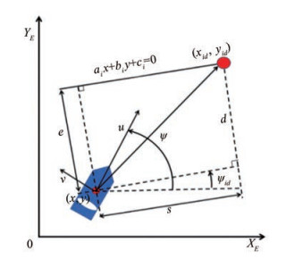Figure  1  USV model

Download: Full-Size Img

where $a_{i}, b_{i}$, and $c_{i} \in \Re$ are the parameters; subscript $i$ denotes the ith route segment. The waypoint $\boldsymbol{p}_{i d}=$ $\left[x_{i d}, y_{i d}\right]^{\mathrm{T}} \in \Re^{2}$ on the route is obtained as follows:

In accomplishing the straight-line following task, waypoint tracking errors are defined as follows:

The time derivative of Equation (13) along the kinematics (9) is given as follows:

where $\beta=\operatorname{atan}(v / u)$ denotes the sideslip angle; $\psi_{i d}=$ $\operatorname{atan} 2\left(-a_{i}, b_{i}\right)$ and $U=\sqrt{u^{2}+v^{2}}$ are the resultant velocity.

As shown in Figure 2, the constrained water region can be modeled as two waterway boundaries $L_{i j}, j=1, 2$ parallel to the ith straight-line route segment. The two waterway boundaries are $L_{i j}=\left\{a_{i j}, b_{i j}, c_{i j} \in \mathfrak{R} \mid a_{i j} x+b_{i j} y+c_{i j}=0, i=\right.$ $1, 2, \cdots, n, j=1, 2\}$. Next, consider $M_{1}$ static obstacles $O_{k s}$, $k=1, 2, \cdots, M_{1}$, which are modeled as a closed circular disk of radius $d_{k s}$, centered at $\boldsymbol{p}_{k s}=\left[x_{k s}, y_{k s}\right]^{\mathrm{T}} \in \Re^{2}$. Consider $M_{2}$ moving obstacles $O_{k m}, k=1, 2, \cdots, M_{2}$, which is modeled as a closed circular disk of radius $d_{k m}$, centered at $\boldsymbol{p}_{k m}=$ $\left[x_{k m}, y_{k m}\right]^{\mathrm{T}} \in \mathfrak{R}^{2}$.

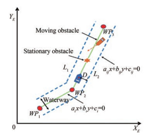Figure  2  Straight-line following of a USV in the constrained water region

Download: Full-Size Img

The safe-certificated straight-line following in a constrained water region aims to design a guidance method for a USV with kinematics (9); that is, the USV is able to converge to the straight-line path and avoid collisions with waterway boundaries and stationary/moving obstacles. In particular, the control objective is divided into four parts.

• The goal reaching task is achieved as follows:

where $\varepsilon_{0} \in \Re$ is a small positive constant.

• Collision avoidance with a waterway boundary task is measured as follows:

where $D_{i j}$ is the distance between USV's center point and the waterway boundary; $L$ is the length of the USV; $W$ is the width of the USV; $d_{i j} \in \Re$ denotes the safe distance between the waterway boundary and the USV.

• Collision avoidance with a stationary obstacle task is measured as follows:

where $d_{k s} \in \Re$ denotes the safe distance between the stationary obstacles and the USV.

• Collision avoidance with a moving obstacle task is calculated as follows:

where $d_{k m} \in \Re$ denotes the safe distance between the moving obstacle and the USV.

3   Design and analysis

As shown in Figure 3 a safety-certificated LOS guidance is designed in this section. First, a straight-line LOS guidance law is developed where an ESO is used to estimate unknown ocean currents. Next, CBFs are constructed to encode currents' collision avoidance tasks of waterway boundaries and stationary/moving obstacles as safety constraints. Finally, quadratic programming problems are formulated to obtain safety-certificated guidance signals within safety and velocity constraints.

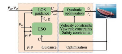Figure  3  Safety-certificated LOS guidance structure

Download: Full-Size Img

3.1   Ocean current ESO design

Let $\hat{w}_{s}$ and $\hat{w}_{e}$ be the estimates of $w_{s}$ and $w_{e}$, respectively. A linear ESO is developed to estimate the unknown ocean as follows:

where $\tilde{s}=\hat{s}-s$ and $\tilde{e}=\hat{e}-e ; k_{s 1}, k_{e 1}, k_{s 2}$, and $k_{e 2} \in \Re$ are positive gains.

Let $\tilde{w}_{s}=\hat{w}_{s}-w_{s}$ and $\tilde{w}_{e}=\hat{w}_{e}-w_{e}$. Consequently, the estimation error dynamics is given as follows:

where $\boldsymbol{E}_{1}=\left[\tilde{s}, \tilde{e}, \tilde{w}_{s}, \tilde{w}_{e}\right]^{\mathrm{T}}, \boldsymbol{w}=\left[\dot{w}_{s}, \dot{w}_{e}\right]^{\mathrm{T}}$ and

Considering that $\boldsymbol{A}$ is a Hurwitz matrix, a symmetric positive definite matrix $\boldsymbol{P}$ is observed; that is, $\boldsymbol{A}^{\mathrm{T}} \boldsymbol{P}+\boldsymbol{P A}=$ - $\xi{\boldsymbol{I}}_{4}$, where $\xi \in \Re$ is a positive constant. In analyzing the stability of (20), the following assumption is made (Gu et al., 2022).

Assumption 1. The disturbances' $w_{i}, i=s, e$ derivatives are bounded; that is, $\left|w_{i}(t)\right|+\left|\dot{w}_{i}(t)\right|<w_{i}^{*}$, with $w_{i}^{*}$ being a positive constant.

Lemma 2. Under Assumption 1, the ESO subsystem (20), with the state vector being $E_{1}$ and the input being $w$, is input-to-state stable (ISS).

Proof: Consider a Lyapunov function

and its time derivative along (20) is given as follows:

As

renders

where $0<\theta_{1}<1$. Therefore, subsystem (20) is ISS (Khalil, 2015), and $\boldsymbol{E}_{1}(t)$ is satisfied as follows:

3.2   LOS guidance design

Before the design, the following assumption is made.

Assumption 2. Considering kinematics, the kinetic error is assumed to be 0, that is, $U=U_{\mathrm{o}}, r=r_{\mathrm{o}}$, where $U_{\mathrm{o}}$ and $r_{\mathrm{o}}$ are the optimized surge velocity and yaw rate, respectively.

Recalling the error dynamics (14),

where $U_{e}=U_{\mathrm{o}}-U_{\mathrm{cmd}}$ and $\psi_{e}=\psi-\psi_{\text {cmd }}$.

By using the estimated information from the ESO (19), a LOS guidance law is designed on the basis of (26).

where $f_{U}=2 U_{\mathrm{o}} \sin ^{2}\left(\frac{\psi-\psi_{i d}+\beta}{2}\right) ; k_{u}>0$ and $k_{r}>0$ are constant controller gains; $\Delta_{u}>0, \Delta_{\psi}>0$ and $\Delta_{r}>0$ are parameters. The velocity guidance signal $U_{\mathrm{cmd}}$ is designed using feedback linearization. The second term of the heading guidance signal $\psi_{\mathrm{cmd}}$ is an LOS angle, which is used to guide the USV converging to the desired path. $g$ is a component additionally designed to compensate for the unknown ocean current in the $e$ direction.

Substituting Equation (27) into Equation (26),

where $G$ is a perturbing term, which is given as follows:

$G\left(\psi_{e}, \psi_{\mathrm{cmd}}, e, U_{\mathrm{o}}\right)$ satisfies $G\left(0, \psi_{\mathrm{cmd}}, e, U_{\mathrm{o}}\right)=0$ and $\|G(\cdot)\| \leqslant \zeta\left(U_{0}\right)\left\|\psi_{e}\right\|$, where $\zeta\left(U_{0}\right)>0$ (Maghenem et al., 2017). $G(\cdot)$ is zero when the perturbing variable $\tilde{\psi}$ is zero, and it has maximal linear growth in perturbing variables.

In compensating for the ocean current component $w_{e}$ in (28), $g$ is selected to satisfy the following equality (Belleter et al., 2019):

Based on (30),

Let $a=\hat{w}_{e}^{2}-U_{0}^{2}, b=e \hat{w}_{e}$ and $c=\Delta_{\psi}^{2}+e^{2}$. Considering that $U_{0}^{2}-\hat{w}_{e}^{2}>0, b^{2}-a c=\Delta_{\psi}^{2}\left(U_{0}^{2}-\hat{w}_{e}^{2}\right)+e^{2} U_{0}^{2}>0$.

Based on the quadratic formula,

where the negative root is abandoned to ensure that $g$ and $\hat{w}_{e}$ have the same sign.

Substituting $g$ into Equation (28), we obtain

Lemma 3. The error subsystem (33), viewed as a system with the states being sand eand the inputs being $\tilde{w}_{s}, \tilde{w}_{e}, U_{e}$, and $G(\cdot)$, is ISS.

Proof: Construct the following Lyapunov function

and its derivative based on (28) is calculated as follows:

where $\bar{k}_{u}=k_{u} / \sqrt{s^{2}+\Delta_{u}^{2}}, \bar{k}_{U o}=U_{0} / \sqrt{(e+g)^{2}+\Delta_{\psi}^{2}}, \boldsymbol{K}=$ $\operatorname{diag}\left\{\bar{k}_{u}, \bar{k}_{U o}\right\}, \boldsymbol{E}_{2}=[s, e]^{\mathrm{T}}, \boldsymbol{h}_{1}=\left[\left|\tilde{w}_{s}\right|+\left|U_{e}\right|, \left|\tilde{w}_{e}\right|+|G(\cdot)|\right]^{\mathrm{T}}$.

As

renders

where $0<\theta_{2}<1$. Consequently, the error subsystem (28) is ISS, and

The time derivative of $\psi_{e}$ is obtained as follows: $\dot{\psi}_{e}=$ $r-r_{\text {cmd }}+r_{\text {cmd }}-\dot{\psi}_{\text {cmd }}$. By substituting (27) into $\dot{\psi}_{e}$, the resulting error system can be expressed as follows:

where $r_{e}=r_{0}-r_{\text {cmdd }}$.

Lemma 4. The error subsystem (39), viewed as a system with the state being $\psi_{e}$ and the inputs being $r_{e}$ and $\dot{\psi}_{\text {cmd }}$, is ISS.

Proof: Construct the following Lyapunov function

and its derivative based on (39) is calculated as follows:

where $\bar{k}_{r}=k_{r} / \sqrt{\psi_{e}^{2}+\Delta_{r}^{2}}$.

As

renders

where $0<\theta_{3}<1$. Consequently, the error subsystem (39) is ISS, and

Lemma 5. The cascaded system formed by subsystem (20), subsystem (33), and subsystem (39) is ISS.

Proof: Based on Lemmas 2 and 3, the ESO subsystem and error subsystem (33) can be considered a cascade system, with the states being $s, e$ and the input being $w$, which is ISS. Based on Lemmas 3 and 4, the error subsystems (33) and (39) can be regarded as a cascade system, with the states being $s, e$ and the inputs being $r_{e}, \dot{\psi}_{\mathrm{cmd}}$, which is ISS. Based on Lemma 4.6 in Khalil (2015), the closedloop system composed of (20), (33), and (39) is ISS.

3.3   CBF design

In this subsection, the collision avoidance of waterway boundaries and stationary/moving obstacles is addressed and encoded as safety constraints by CBFs. Then, a quadratic optimization problem is established to optimize the command signals obtained in Section 3.2.

3.3.1   CBF design for avoiding stationary obstacles

Let $\boldsymbol{p}_{k s}=\left[x_{k s}, y_{k s}\right]^{\mathrm{T}}$ be the position of the stationary obstacles. In avoiding the stationary obstacles, the following CBF for the collision avoidance of stationary obstacles is constructed:

Recalling (9), it follows that

where $\left[\hat{w}_{x}, \hat{w}_{y}\right]^{\mathrm{T}}=\underline{R}\left(\psi_{i d}\right)\left[\hat{w}_{s}, \hat{w}_{e}\right]^{\mathrm{T}}\left[\tilde{w}_{x}, \tilde{w}_{y}\right]^{\mathrm{T}}=\underline{R}\left[\tilde{w}_{s}, \tilde{w}_{e}\right]^{\mathrm{T}}$ and

Using (8), the second time derivatives of $h_{k s}$ in (44) can be expressed as follows:

and the corresponding constraints are expressed as follows:

where

and $\alpha_{s} \in \Re$ is a positive constant.

3.3.2   CBF design for avoiding moving obstacles

In avoiding the moving obstacles, the following $\mathrm{CBF}$ is constructed as follows:

Using (8), the time derivatives of $h_{k m}$ in (48) can be expressed as follows:

and the corresponding constraints are expressed as follows:

where

and $\alpha_{m} \in \Re$ is a positive constant.

Remark 1: Based on Rule 9(e) of the International Regulations for Preventing Collisions at Sea (COLREGS), in a narrow waterway or fairway, overtaking can only occur if the vessel to be overtaken takes action to permit safe passing. Otherwise, overtaking behavior is not permitted. This paper considers the situation in that USV is not allowed to overtake, and it has to follow the vessel ahead at a low speed. Hence, the speed is optimized to avoid collisions with the vessel ahead.

3.3.3   CBF design for avoiding waterway boundaries

The boundaries of the waterway are represented by two straight lines, denoted by $L_{i j}$ (Figure 4), and their expressions are defined as follows:

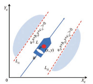Figure  4  Schematic diagram of the waterway boundary constraints

Download: Full-Size Img

where $a_{i j}, b_{i j}$, and $c_{i j} \in \Re$ are the parameters of the line.

Based on the property of (51), the area where the two straight lines are larger than zero is defined as a safety set for the USV, and the safety area $\mathcal{C}$ can be expressed as follows:

The distance between the USV and the waterway boundary is defined as follows:

In ensuring the safety, the safety set is defined as follows:

indicating that the distance between each edge of the USV and the waterway boundaries should be larger than distance $d_{i j}$. By using (8), the second time derivatives of $h_{i j}$ in (53) can be expressed as follows:

and the corresponding waterway boundary constraints are expressed as follows:

where

and $\alpha_{c} \in \Re$ is a positive constant.

3.4   Safety-certificated guidance law design

By using the safety constraints determined by CBFs, two quadratic programming problems are formulated herein to optimize the obtained guidance law in a minimal invasion way to ensure the safety of the USV. In addition, the following velocity constraints are enforced to satisfy the following equation:

where $\underline{U} \in \Re, \bar{U} \in \Re, \underline{r} \in \Re$, and $\bar{r} \in \Re$ are constants.

The optimized velocity $U_{0}$ is obtained by solving the following quadratic programming problem:

Similarly, the optimized yaw rate $r_{\mathrm{o}}$ is obtained as follows:

The safety of the USV system is given by the following lemma.

Lemma 6. Given an under-actuated USV with dynamics (9), if the optimal control signal $U_{0} \in \mathcal{U}_{2}$ and $r_{0} \in \mathcal{U}_{1} \cap \mathcal{U}_{3}$ for the USV, and $\boldsymbol{p}\left(t_{0}\right) \in \mathcal{S}_{1} \cap \mathcal{S}_{2} \cap \mathcal{S}_{3}, \forall t>t_{0}$, then, the USV system is ISSf.

Proof: The set $\mathcal{S}=\mathcal{S}_{1} \cap \mathcal{S}_{2} \cap \mathcal{S}_{3}$ is forward invariant by using the optimal control signal $U_{0} \in \mathcal{U}_{2}$ and $r_{0} \in \mathcal{U}_{1} \cap \mathcal{U}_{3}$; that is, the set $\mathcal{S}$ is ISSf. Therefore, if the initial position of the USV satisfies $\boldsymbol{p}\left(t_{0}\right) \in \mathcal{S}_{1} \cap \mathcal{S}_{2} \cap \mathcal{S}_{3}$, then $\boldsymbol{p}(t)$ will stay in $\mathcal{S}_{1} \cap \mathcal{S}_{2} \cap \mathcal{S}_{3}$. Therefore, the USV system is ISSf.

The stability and safety of the proposed system of USV are given by the following theorem.

Theorem 1. Consider a USV with dynamics (9), the ESO (19), safety constraints (47), (50), and (55), optimal surge velocity (57), and optimal yaw rate (58). All error signals in the closed-loop system are uniformly and ultimately bounded, and the USV system is ISSf.

Proof: Based on Lemma 6, the USV will not violate the safety requirements; that is, the safety objectives (16), (17), and (18) are achieved. Lemma 3 shows that the tracking error signal $\boldsymbol{E}_{2}$ is bounded; that is, there exists a positive constant such that the geometric objective (15) is achieved.

4   Simulation of a USV in the yangtze river

Consider a motion scenario that a USV runs in the waterway of the Yangtze River. Moreover, consider one sta- tionary obstacle and one moving obstructive vehicle running at a low velocity ahead of the USV.

In the simulation, the length and width of the USV are set as $L=1.5$ and $W=0.4$, respectively. The ocean currents are set as $w_{s}=-0.5$ and $w_{e}=0.2$. The velocity constraints are given as $\underline{U}=0, \bar{U}=1, \underline{r}=-0.5$, and $\bar{r}=0.5$. The initial position of the USV is $\boldsymbol{p}(0)=[2, 72.5]^{\mathrm{T}}$. The desired straight lines are determined by three waypoints, that is, $\boldsymbol{p}_{1 d}=[0, 72.5]^{\mathrm{T}}, \boldsymbol{p}_{2 d}=[21.6, 60.0]^{\mathrm{T}}$, and $\boldsymbol{p}_{3 d}=[88.0, 0]^{\mathrm{T}}$. The parameters of the four waterway boundaries are $119 x+$ $195 y-13494=0, -152 x-233 y+17800.2=0, 573 x+$ $635 y-47559=0$, and $-566 x-662 y-53852.8=0$. The stationary obstacle locates $\boldsymbol{p}_{1 s}=[34.0, 50.0]^{\mathrm{T}}$. The obstructive vehicle moves at a speed of $0.7 \mathrm{~m} / \mathrm{s}$ on the route. The safe distances are set as follows:

The ESO parameters are selected as $k_{s 1}=1, k_{e 1}=1$, $k_{s 2}=0.25$, and $k_{e 2}=0.25$. The LOS guidance parameters are selected as $k_{u}=1, \Delta_{u}=0.5, \Delta_{\psi}=8, k_{r}=0.5$, and $\Delta_{r}=0.3$. The CBF parameters are set as $\alpha_{c}=0.5$, $\alpha_{s}=0.45$, and $\alpha_{m}=0.05$. In the simulation, the quadratic optimization problem is solved by the built-in Python toolbox cvxpy.

The simulation results are provided in Figures 5-9. Figure 5(a) shows the simulation results of the proposed guidance method. Compared with Figure 5(b), safety is ensured; that is, the collisions with waterway boundaries and obstacles are prevented by using the proposed CBF-based guidance method. Compared with Figure 5(c), the USV can accurately track the desired route by using the proposed ESO-based guidance method. Figure 6 shows the tracking errors of the USV in the $s$ and $e$ directions. Based on the error shown in the $s$ direction, the proposed method and the method without ESO can reduce the velocity when encountering a moving obstacle. Based on the error in the $e$ direction, the error cannot be eliminated by using the method without ESO as the effect of unknown ocean currents. Figure 7 shows the estimation performance of the ocean current ESO. The unknown constant ocean currents are estimated accurately. Figure 8 shows the yaw rate tracking performance. The commanded yaw rate is optimized at $0-20 \mathrm{~s}$ and $70-80 \mathrm{~s}$ to ensure the collision avoidance of waterway boundaries and obstructive vehicles, respectively. The peak at $50 \mathrm{~s}$ is induced by the change of the desired straight-line route. Figure 9 shows the surge velocity tracking performance. The peak at $50 \mathrm{~s}$ is also induced by the change of the desired straight-line route. Considering the role of CBF, the USV can decelerate after $130 \mathrm{~s}$ because of the presence of a moving vessel in front of it. Figure 10 shows the quadratic programming time for the surge and yaw directions. The optimization time is less than the sampling time $\Delta T$ in each cycle, which can be accomplished in each cycle. Figure 11 shows the ratio of the quadratic programming time to the total execution time in each cycle. As shown in the figure, optimization occupies more than $90 \%$ of the total execution time in each cycle.

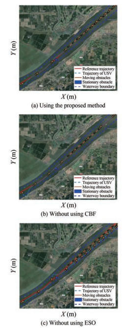Figure  5  USV trajectory

Download: Full-Size Img

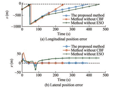Figure  6  Comparison of position errors using three methods

Download: Full-Size Img

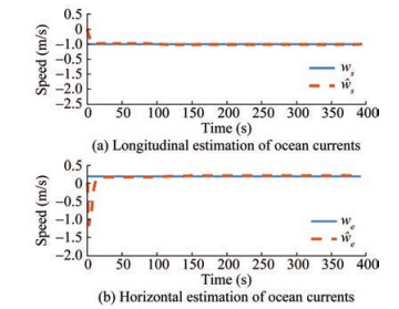Figure  7  Estimation performance of the ESO

Download: Full-Size Img

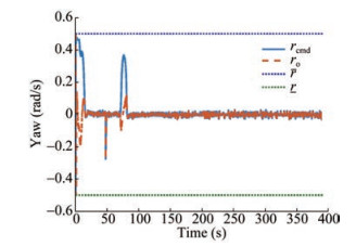Figure  8  Commanded yaw rate and optimized yaw rate command

Download: Full-Size Img

Figure  9  Commanded surge speed and optimized surge speed command

Download: Full-Size Img

Figure  10  Quadratic programming time

Download: Full-Size Img

Figure  11  Ratio of the quadratic programming time to the total execution time in each cycle

Download: Full-Size Img

5   Conclusion

This paper presents a safety-certified straight-line following of a USV in a constrained water region with waterway boundaries and stationary/moving obstacles. An ESO is designed to estimate external environmental disturbances. Design guidance laws based on the principle of LOS, and compensate for external disturbances based on the ESO results. Then, a quadratic programming problem is formulated such that the safety constraints encoded by CBFs and velocity constraints are satisfied. Therefore, all tracking errors of the closed-loop system are uniformly and ultimately bounded, and the system is ISSf. The simulation results substantiate the effectiveness of the proposed safety-certified straight-line following guidance method. In future work, the USV dynamic model must be considered, and the antidisturbance safe-certificated path following control must be investigated for a USV in a constrained water region.