Fractional Super-Twisting/Terminal Sliding Mode Protocol for Nonlinear Dynamical Model: Applications on Hovercraft/Chaotic Systems
https://doi.org/10.1007/s11804-023-00329-7
-
Abstract
Fractional terminal and super-twisting as two types of fractional sliding mode controller are addressed in the present paper. The proposed methodologies are planned for both the nonlinear fractional-order chaotic systems and the nonlinear factional model of Hovercraft. The suggested procedure guarantees the asymptotic stability of fractional-order chaotic systems based on Lyapunov stability theorem, by presenting a set of fractional-order laws. Compared to the previous studies that concentrate on sliding mode controllers with unwanted chattering phenomena, the proposed methodologies deal with chattering reduction of terminal sliding mode controller/super twisting to converge to desired value in finite time, consequently. The main advantages of the offered controllers are 1) closed-loop system stability, 2) robustness against external disturbances and uncertainties, 3) finite time zero-convergence of the output tracking error, and 4) chattering phenomena reduction. Finally, the simulation results show the performance of the approaches both on the chaotic and Hovercraft models.Article Highlights● Fractional super-twisting sliding mode control (SMC) is developed for fractional nonlinear model of hovercraft.● Terminal SMC is derived for fractional nonlinear model of hovercraft.● Convergence of the tracking error to zero in finite time is guaranteed. -
1 Introduction
Fractional calculus background dates to the seventeenth century, and the Hopital letter goes back to Leibniz and asked his opinion about the derivative of the fractional-order 0.5. Subsequently, the researchers propose definitions for the fractional-order derivative and integral to apply on their applications. Nowadays, fractional calculus has several applications in various sciences (Podlubny, 1998). Robotic (Couceiro et al., 2010; Munoz et al., 2007), bioengineering (Magin, 2006), cancer disease (Rook and Ghasemi, 2018), signal processing (Aslam and Raja, 2015), chaos phenomena (Rabah et al., 2017; Tavazoei et al., 2008), controllers design (Sira-Ramírez, 2002), and observers design (Sharafian and Ghasemi, 2019) are some of the application for the fractional calculus. The fractional models because of their accuracy than the integer-order ones are attract scientists and engineering to describe real objects (Petras, 2010).
Hovercraft, as an amphibious craft, are capable to travel over land, water, and other faces. British inventor Christopher Cockrell constructed the first real-world Hovercraft in the 1950s. Due to their exceptional features, they have unique capabilities in various areas. The crucial application of Hovercraft is the transportation of tanks, soldiers, and large equipment in hostile environments (Cabecinhas et al., 2017; Modiri and Mobayen, 2020).
The chaos behavior is the characteristic structure of fractional dynamical models. In recent decades, chaos has been raised as one of the quarrelsome subjects in engineering, physics, and mathematics and furthermore their researches have grown extremely. The chaos has a random appearance due to its name, which occurs in many of phenomena. The famous phenomenon is the specific feature of chaos as "butterfly effect". In 1963, the Meteorologist "Edward Lorenz" acquired the first chaotic 3rd-order dynamic (Lorenz, 1963). Because of the complex dynamics and inherent instability of the chaotic system, it was first thought that chaotic systems couldn't be controlled. In 1990, it was shown that chaotic systems are controllable and various control objectives can be considered for them (Ott et al., 1990).
One of the famous techniques for designing a robust controller is chaotic systems sliding mode control (SMC). The overall structure of SMC is simple and fast responding, without sensitivity respect to external disturbances and internal parameters (Utkin, 1992). Chattering phenomenon is inherent in the traditional sliding mode controller due to its discontinuity nature. To reduce the chattering and to keep the advantages of traditional SMC, high order one is suggested in Levantovsky and Levant (1987). For high order sliding mode, a popular applicable approach is the super-twisting algorithm. In Sharafian and Ghasemi (2019), an observer of Neuro-terminal sliding mode has been designated for an affine nonlinear system. Fractional nonsingular terminal SMC is offered in Shahbazi et al. (2021) regarding a nonlinear fractional-order class of chaotic systems. To control of Hovercraft, the following references can be mentioned. A reinforcement learning based tracking controller based on inputs/outputs of the USV in Wang et al. (2021). In Wang and Su (2019), a finite-time observer-based interactive trajectory tracking control scheme is created for an asymmetric under-actuated surface vehicle.
Hu et al. (2020) addresses terminal SMC regarding a nonlinear class of fractional second order system. Fractional variable structure fuzzy SMC for nonlinear systems is derived in Song et al. (2018) based on finite time stability in presence of uncertainties. Adaptive SMC is developed for fractional order TS observer in Li and Zhang (2022). Djeghali et al. (2021) depicts sliding mode disturbance observer for uncertain fractional nonlinear systems. Alipour et al. (2022) deals with fractional nonsingular terminal SMC to apply on spacecraft model.
L1 adaptive back stepping approach is developed in XU et al. (2021) for path planning of nonlinear model of under actuated ship with guaranteed stability. Xu et al. (2020) deal with the sliding mode heading autopilot with guaranteed exponentially stable approach. This procedure should be applied in unmanned vehicles such as aircraft, underwater vehicles, drones and autonomous vehicles.
Our approach focuses on the super twisting/terminal sliding mode controller (STSMC and TSMC) design regarding the special chaotic system class of nonlinear fractional-order (FO). Our methodology has some merits such as: 1) convergence of tracking error to zero, 2) the closed-loop system stability, and 3) reduction of the chattering phenomena. For proving the convergence of STSMC and TSMC algorithms, Lyapunov function is used.
The organization of the present paper is explained next. A basic definition of fractional calculus (covering the fractional integral and differential) is included in section 2, then models the Hovercraft, and describes the special fractional order system. As a nonlinear fractional system class, a super twisting sliding mode controller is introduced in section 3. Section 4 depicts fractional terminal sliding mode procedure design. Section 5 presents the simulation results of the proposed methods applied on the chaotic fractional system and Hovercraft. Finally, section 6 involves brief conclusions.
2 Preliminaries and system formulation
In this part, some basic definitions, preliminaries of fractional calculus, hovercraft model, and a special class of FO system are all given.
2.1 Fractional Mathematics
Three common definitions of fractional-order derivative and a fractional integral are designate in the following in Podlubny (1998).
Definition 1:The Grunwald-Letnikov (G) derivative definition of order $q$ of function $f(t)$ is described as:
$$ { }_{a}^{\mathrm{GL}} D_{t}^{q} f(t)=\lim _\limits{N \rightarrow \infty}\left[\frac{t-a}{N}\right]^{-q} \sum\limits_{j=0}^{N-1}(-1)^{j}\left(\begin{array}{l}q \\ j\end{array}\right) f\left(t-j\left[\frac{t-a}{N}\right]\right) $$ Definition 2: Riemann-Liouville (RL) FO integral and derivative is one of the most popular definitions. The RL integral of order $q$ is defined as,
$$ { }_{a} D_{t}^{-q} f(t)=\frac{1}{\mathit \Gamma(q)} \int_{a}^{t}(t-\tau)^{q-1} f(\tau) \mathrm{d} \tau $$ and the RL derivative of order $\mathrm{q}$ is:
$$ { }_{a}^{\mathrm{RL}} D_{t}^{q} f(t)=\frac{1}{\mathit \Gamma(1-q)} \frac{\mathrm{d}}{\mathrm{d} t} \int_{a}^{t}(t-\tau)^{-q} f(\tau) \mathrm{d} \tau $$ (1) where the Gamma function is depicted by $\mathit \Gamma(\cdot)$ and $0<$ $q<1$
Definition 3: The $q$-order derivative of Caputo (C) type is given by:
$$ { }_{a}^{c} D_{t}^{q} f(t)=\frac{1}{\mathit \Gamma(1-q)} \int_{a}^{t}(t-\tau)^{-q} \dot{f}(\tau) \mathrm{d} \tau $$ (2) Some properties of fractional derivatives are as follows:
Fractional differentiation is linear operation (Petras, 2010):
$$ { }_{a} D_{t}^{q}(\alpha f(t)+\beta g(t))=\alpha_{a} D_{t}^{q} f(t)+\beta_{a} D_{t}^{q} g(t) $$ (3) Take the derivable and continuous function of $x(t) \in \mathbb{R}$ in- to assumption. In every time instant $t \geqslant t_{0}$ and $0<q<1$
$$ \frac{1}{2}{ }_{t_{0}}^{C} D_{t}^{q} x^{2}(t) \leqslant x(t){ }_{t_{0}}^{C} D_{t}^{q} x(t) $$ (4) The solution of ${ }_{0}^{c} D_{t}^{q} x(t)=f(t, x)$, Mittag-Leffler stability (Li et al., 2009) was considered as Mittag-Leffler stable in the case of
$$ \|x(t)\| \leqslant\left\{m\left[x\left(t_{0}\right)\right]\left(t-t_{0}\right)^{-\gamma} E_{\alpha, 1-\gamma}\left(-\lambda\left(t-t_{0}\right)^{\alpha}\right)\right\}^{b} $$ (5) where $m(x)$ (with Lipschitz constant $m_{0}$) is Lipschitz locally on $x \in B \in \mathbb{R}^{n}, m(x) \geqslant 0, m(0)=0, b>0, \lambda \geqslant 0$, $\gamma \in[0, 1-\alpha], \alpha \in(0, 1)$, and the initial time is represented by $t_{0}$.
Remark 1: Asymptotic stability is implied by MittagLeffler stability (Li et al., 2009).
Theorem 1: As an equilibrium point in system ${ }_{0}^{c} D_{t}^{q} x(t)=f(t, x)$ consider $x=0$. Also, as a domain containing the origin take $D \subseteq \mathbb{R}$ into consideration. As a continuous differentiable function presume $V(t, x(t))$ : $[0, \infty) \times D \rightarrow \mathbb{R}$ which is Lipschitz locally respecting $x$ in a way that
$$ \begin{gathered} \alpha_{1}\|x\|^{a} \leqslant V(t, x(t)) \leqslant \alpha_{2}\|x\|^{a b} \\ { }_{0}^{c} D_{t}^{\beta} V(t, x(t)) \leqslant-\alpha_{3}\|x\|^{a b} \end{gathered} $$ (6) where $t \geqslant 0, x \in D, \beta \in(0, 1), \alpha_{1}, \alpha_{2}, \alpha_{3}, a$ and $b$ represent positive constants of arbitrary type. Hence, the Mittag-Leffler stable equation of $x=0$ is considerable. This equation would be globally Mittag-Leffler stable if hypotheses hold on $\mathbb{R}^{n}$ globally (Li et al., 2009).
In this paper, we use Caputo fractional order operators as our main tool.
2.2 Hovercraft Modelling
The Hovercraft controller design is a so attractive subject for researchers. These controller procedures are so complicated due to 1) high speed, 2) low friction, 3) nonholonomic constraint of $2^{\text {nd }}$ order on dynamics, 4) heading path force generation in actuators, 5) dynamical coupling among states. The symbols and their descriptions of Hovercraft dynamics are shown in Table 1 (Jeong and Chwa, 2017).
Figure 1 depicts Hovercraft model in a two-dimensional space as a rigid body frame $\{B\}$ and inertial frame $\{I\}$.
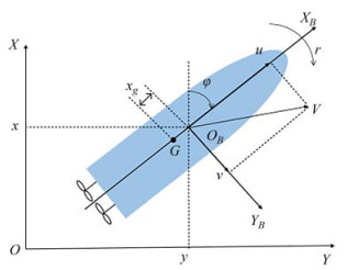 Figure 1 Outline of hovercraft model
The kinematics and dynamics of the hovercraft are as follows:
$$ \left\{\begin{array}{l} D^{q} x=\cos (\theta) u-\sin (\theta) v \\ D^{q} y=\sin (\theta) u+\cos (\theta) v \end{array}\right. $$ (7) Table 1 The symbols of hovercraft dynamicsSymbol Explanation $ a $ The arm length from mass center to the surface of rudder $ v $ Lateral velocity $ r $ Angular velocity $ \theta $ Rudder angle $ T $ Trust force $\left\{u_d, v_d, x_d, y_d\right\}$ Desired parameters $\left\{d_{u_0}, d_{v_0}, d_{r_0}, d_u, d_v, d_r\right\}$ Friction coefficients $ m $ Mass of hovercraft $ J $ Inertia moment $ u $ Longitudinal velocity $\left[\begin{array}{cc} \cos \theta & \sin \theta \\ -\sin \theta & \cos \theta \end{array}\right]$ Rotational matrix (ex, ey) Position tracking errors (eu, ev) Velocity errors bT Force scaling coefficient $$ \left\{\begin{array}{l} D^{q} u=-m^{-1} d_{u_{0}} \operatorname{sign}(u)-m^{-1} d_{u} u+m^{-1} b_{T} T \cos (\theta)+v r \\ D^{q} v=-m^{-1} d_{v_{0}} \operatorname{sign}(v)-m^{-1} d_{v} v+m^{-1} b_{T} T \sin (\theta)-u r(8) \\ D^{q} r=-J^{-1} d_{r_{0}} \operatorname{sign}(r)-J^{-1} d_{r} r-J^{-1} a b_{T} T \cos \end{array}\right. $$ (8) where $x, y, u, v$, and $r$ stand for positions, longitudinal, lateral, and angular velocity, respectively. $M$ and $T$ show the mass of Hovercraft and trust force.
2.3 Problem formulation
In this section, we introduce a wide class of nonlinear FO systems as:
$$ \left\{\begin{array}{l} D^{q} x=F_{1}(x, y, z) \\ D^{q} y=F_{2}(x, y, z)+u(t)+\sigma(t) \\ D^{q} z=F_{3}(x, y, z) \end{array}\right. $$ (9) where $u$ is the control input, the state variable is represented by $\boldsymbol{x}=[x, y, z]^{\mathrm{T}}, F_{1}, F_{2}$, and $F_{3}$ show nonlinear function, and $\sigma(t)$ represents the uncertainties. Some systems such as Chen, Liu, Lu, and Lorenz chaotic model can be presented in the form of the Equation (9).
If we consider $F_{1}(x, y, z)=a(y-x), F_{2}(x, y, z)=c x-$ $x z-y$ and $F_{3}(x, y, z)=x y-b z$, then the system shows the Lorenz chaotic system.
To track the desired trajectory, custom SMC uses linear sliding-mode (LSM) surface. In LSM controller design, the main challenge is the selection of sliding surface according to the requirements of system performance.
3 Procedure design of fractional supertwisting sliding mode
The first step in the sliding mode control procedure is designating a sliding surface.
$$ s=x+\lambda_{1} y+\lambda_{2} z $$ (10) where $\lambda_{1}$ and $\lambda_{2}$ are positive constants. According to Equation (5), by assuming the mentioned equation's fractional $q$-order differential and using Equation (9), we have:
$$ \begin{aligned} D^{q} S & =D^{q} x+\lambda_{1} D^{q} y+\lambda_{2} D^{q} z \\ & =F_{1}(x, y, z)+\lambda_{1} F_{2}(x, y, z)+\lambda_{2} F_{3}(x, y, z) \end{aligned} $$ (11) The second step in the SMC procedure is the introduced control signal. The control objectives are both the stability of closed-loop system and the chattering-free zero-convergence of the sliding surface. To guarantee this goal, the super twisting SMC law is suggested as:
$$ u(t)=u_{\mathrm{eq}}(t)+u_{r}(t) $$ (12) where the $u_{\mathrm{eq}}(t)$ and $u_{r}(t)$ reach controller parts equally based on the following definitions.
$$ \begin{aligned} u_{\mathrm{eq}}(t)= & \frac{1}{\lambda_{1}}\left[-F_{1}(x, y, z)-\lambda_{1} F_{2}(x, y, z)-\right. \\ & \left.\lambda_{2} F_{3}(x, y, z)-\lambda_{1} \sigma(t)\right] \end{aligned} $$ (13) and $u_{r}(t)$ is as below
$$ u_{r}(t)=\frac{1}{\lambda_{1}}\left[-\alpha|s|^{\rho} \operatorname{sgn}(s)-\beta \int \operatorname{sgn}(s) \mathrm{d} t\right] $$ (14) Compensation of model uncertainties are performed by the 1 st term. The other term is responsible for decreasing the phenomena of chattering where the $\alpha, \beta, \rho$ in Equation (14) satisfy $0<\rho<1$ and $\alpha, \beta>0$.
The below theorem is derived by the authors, to comfort the super twisting sliding mode controller design.
Theorem 2: Consider the nonlinear FO system mentioned in Equation (9) and the sliding surface designated by Equation (10). The controller structure proposed in (12), (13), and (14) make the closed-loop system stable in the sense of the Lyapunov and bounded all signals involved in it.
Proof: To investigate the stability of a closed-loop system, the next Lyapunov function is considerable.
$$ V=\frac{1}{2} s^{2} $$ (15) Using Equation (6), the derivative of order $q$ in the former equation is
$$ D^{q} V \leqslant s \cdot D^{q} s $$ (16) According to Equation (11), expression (16) can be written that
$$ \begin{aligned} D^{q} V \leqslant & s \cdot D^{q} s=s\left[D^{q} x+\lambda_{1} D^{q} y+\lambda_{2} D^{q} z\right]= \\ & s\left[F_{1}(x, y, z)+\lambda_{1} F_{2}(x, y, z)+\right. \\ & \left.\lambda_{1} \sigma(t)+\lambda_{1} u+\lambda_{2} F_{3}(x, y, z)\right] \end{aligned} $$ (17) By Equations (12) through (14), the Equation (17) can be reconstructed as:
$$ D^{q} \mathrm{~V} \leqslant-\alpha|s|^{\rho+1}-\beta \int|s| \leqslant 0 $$ (18) Based on the theorem 1, it concludes the closed-loop stability; and accordingly, the sliding surface converges to zero. Furthermore, it is assured that signals in the closedloop system are bounded. Thus the proof is completed.
In the simulation results section, the application of the proposed method to the chaotic systems class is demonstrated to depict the capability of the mentioned controller.
4 Fractional terminal sliding mode procedure design
Consider the $e_{u}=u-u_{d}$ and $e_{v}=v-v_{d}$ as the velocity errors. Using $e_{x}=x-x_{d}$ and $e_{y}=y-y_{d}$ as the position error, the $u_{d}$ and $v_{d}$ as desired value of longitudinal, lateral can be derived below.
$$ \left[\begin{array}{l} u_{d} \\ v_{d} \end{array}\right]=\left[\begin{array}{cc} \cos \psi & \sin \psi \\ -\sin \psi & \cos \psi \end{array}\right]\left[\begin{array}{l} D^{q} x_{d}+l_{x} \tanh \left(-k_{x} e_{x}\right) \\ D^{q} y_{d}+l_{y} \tanh \left(-k_{y} e_{y}\right) \end{array}\right] $$ (19) where $k_{x}, k_{y}, l_{x}$, and $l_{y}$ are positive scalar.
Theorem 3: Convergence of the $e_{u}$ and $e_{v}$ as velocity er- rors to zero makes the position errors $\left(e_{x}, e_{y}\right)$ converge to the origin asymptotically.
Proof: Equation (20) is gained using kinematics mentioned in (8).
$$ \left[\begin{array}{l} u \\ v \end{array}\right]=\left[\begin{array}{cc} \cos \psi & \sin \psi \\ -\sin \psi & \cos \psi \end{array}\right]\left[\begin{array}{l} D^{q} x \\ D^{q} y \end{array}\right] $$ (20) Substituting Equations (19) and (20) to the velocity errors, $e_{u}$ and $e_{v}$ can be reconstructed as:
$$ \begin{aligned} {\left[\begin{array}{l} e_{u} \\ e_{v} \end{array}\right]=} & {\left[\begin{array}{l} u \\ v \end{array}\right]-\left[\begin{array}{l} u_{d} \\ v_{d} \end{array}\right]=} \\ & {\left[\begin{array}{cc} \cos \psi & \sin \psi \\ -\sin \psi & \cos \psi \end{array}\right]\left[\begin{array}{l} D^{q} e_{x}-l_{x} \tanh \left(-k_{x} e_{x}\right) \\ D^{q} e_{y}-l_{y} \tanh \left(-k_{y} e_{y}\right) \end{array}\right] } \end{aligned} $$ (21) The Equation (22) is obtained when both $e_{u}$ and $e_{v}$ converge to zero.
$$ \left\{\begin{array}{l} D^{q} e_{y}=l_{y} \tanh \left(-k_{y} e_{y}\right) \\ D^{q} e_{x}=l_{x} \tanh \left(-k_{x} e_{x}\right) \end{array}\right. $$ (22) Candidate the following Lyapunov function to demonstrate the overall stability of the closed loop system.
$$ V_{e}=\frac{1}{2} e_{x}^{2}+\frac{1}{2} e_{y}^{2} $$ (23) Taking $q$-order time derivative of Equation (23) leads to the Equation (24).
$$ D^{q} V_{e} \leqslant e_{x} D^{q} e_{x}+e_{y} D^{q} e_{y} $$ (24) Using Euation (22), we have
$$ D^{q} V_{e} \leqslant-l_{x} e_{x} \tanh \left(k_{x} e_{x}\right)-l_{y} e_{y} \tanh \left(k_{y} e_{y}\right) $$ (25) Let $l_{x}, l_{y}, k_{x}, k_{y}$ be positive constant parameters; then it is obvious $D^{q} V_{e} \leqslant 0$ and position errors $\left(e_{x}, e_{y}\right)$ converge to zero neighborhood.
This completes the proof.
The first step in the terminal sliding mode control procedure is designating a sliding surface as:
$$ s=e_{u}+\lambda e_{v}^{\alpha} $$ (26) where $\lambda>0, \alpha<1$.
Taking the $q$-order time derivative of Equation (26) and using Equations (5) and (8) leads to the following equation.
$$ \begin{aligned} D^{q} s= & D^{q} e_{u}+\frac{\lambda \Gamma(\alpha+1)}{\Gamma(\alpha-q+1)} e_{v}^{\alpha-q} D^{q} e_{v}=\left(D^{q} u-D^{q} u_{d}\right)+ \\ & \frac{\lambda \Gamma(\alpha+1)}{\Gamma(\alpha-q+1)} e_{v}^{\alpha-q}\left(D^{q}-D^{q} v_{d}\right) \\ D^{q} s= & \left(-m^{-1} d_{u_{0}} \operatorname{sign}(u)-m^{-1} d_{u} u+m^{-1} b_{T} T \cos (\theta)+v r-D^{q} u_{d}\right) \\ & +\frac{\lambda \Gamma(\alpha+1)}{\Gamma(\alpha-q+1)} e_{v}^{\alpha-q}\left(-m-d_{v_{0}} \operatorname{sign}(v)-m^{-1} d_{v} v+\right. \\ & \left.m^{-1} b_{T} T \sin (\theta)-u r-D^{q} v_{d}\right) \end{aligned} $$ (27) To guarantee both the finite time stability and the disturbance rejection, the TSMC law is proposed as:
$$ \begin{gathered} T=\left(m^{-1} b_{T}\right)^{-1}\left[m^{-1} d_{u_{0}} \operatorname{sign}(u)+m^{-1} d_{u} u-v r+D^{q} u_{d}\right. \\ \left.\quad-K_{1} \operatorname{sign}(s)\right] \\ \theta=\left(\frac{\lambda \Gamma(\alpha+1) b_T}{m \Gamma(\alpha-q+1)} e_v^{\alpha-q}\right)^{-1}\left[m^{-1} d_{v_o} \operatorname{sign}(v)\right. \\ \left.+m^{-1} d_v v+u r+D^q v_d-K_2 \operatorname{sign}(s)\right] \end{gathered} $$ (28) Theorem 4: Consider Hovercraft dynamics mentioned in Equation (8). Then the sliding surface proposed in equation (26) and control inputs discussed in Equation (28) cause the asymptotic stability of the closed loop system. Besides, the zero-convergence of sliding surface and tracking errors is satisfied, and bounds for all system signals would be determinable.
Proof: Lyapunov function is candidate as
$$ V_{s}=\frac{1}{2} s^{2} $$ (29) The $q$-order derivative of the Equation (29) is
$$ D^{q} V_{s} \leqslant s \cdot D^{q} s $$ (30) Substituting Equation (27) in Equation (30), we have
$$ \begin{aligned} D^{q} V_{s} & \leqslant s \cdot\left[\left(-m^{-1} d_{u_{0}} \operatorname{sign}(u)-m^{-1} d_{u} u+\right.\right. \\ & m^{-1} b_{T} T \cos (\theta)+v r-D^{q} u_{d}+ \\ & \frac{\lambda \Gamma(\alpha+1)}{\Gamma(\alpha-q+1)} e_{v}{ }^{\alpha-q}-m^{-1} d_{v_{0}} \operatorname{sign}(v)-m^{-1} d_{v} v+ \\ & \left.\left.m^{-1} b_{T} T \sin (\theta)-u r-D^{q} v_{d}\right)\right] \end{aligned} $$ (31) Using control inputs in (28), the Equation (31) can be rewritten as
$$ D^{q} \mathrm{~V} \leqslant s\left(-K_{1} \operatorname{sign}(s)-K_{2} \operatorname{sign}(s)\right) \leqslant 0 $$ (32) This completes the proof.
5 Simulation results
To check the suggested control procedures efficiency and capability, this section deals with the application of the cases.
Case 1: Chaotic System
Suppose the following nonlinear FO Lorenz system.
$$ \left\{\begin{array}{l} D^{q} x=a(y-x) \\ D^{q} y=c x-x z-y+u(t)+\sigma(t) \\ D^{q} z=x y-b z \end{array}\right. $$ (33) where $(a, b, c)=\left(10, \frac{8}{3}, 28\right)$ and $\sigma(t)=\sin (w t)$ as an external disturbance.
Next, Figure 2 is obtained for both $[x(0), y(0), z(0)]=$ $[1, 5, 4]$ as initial conditi ons and $[x(0), y(0), z(0)]=$ $[-9, -1, 9]$ in order to depict the extreme chaotic performance of Equation (33).
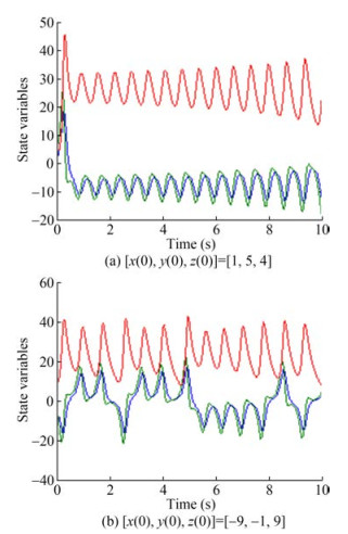 Figure 2 Original system's state variable
Employing the suggested controller in Equation (12), Figure 3 shows the states of the system.
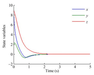 Figure 3 Proposed method's state variable with $[x(0), y(0), z(0)]=$ $[9, 1, 9]$
According to the results of the simulation, the comparison of Figures 1 and 2 depicts the zero-convergence of the states of the system asymptotically without chattering (Figure 3).
Figure 4 demonstrates the sliding surface's smoothness tending to zero.
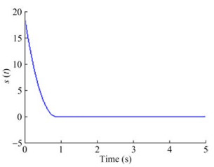 Figure 4 The proposed sliding surface trajectory
Figure 5 shows that the control signal without chattering. The simulation outcomes illustrate promising performances in both tracking and stability approach. The proposed controller succeeds in chattering reduction.
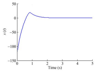 Figure 5 Proposed control input
The capability performance of the proposed model is observable in Figures 2-6. According to the Comparison of our technique with Aghababa (2013), based on Figures 3-6, the planned approach guarantees 1 - the faster convergence to zero, 2- robustness against disturbances.
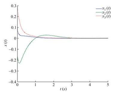 Figure 6 State variable (Aghababa, 2013)
Case 2: Hovercraft
As an illustration of the proposed procedure mentioned in sections 3, 4, the Hovercraft is simulated with the aid of friction coefficients and parameters of Karami and Ghasemi (2020). The Hovercraft mass was $0.585 \mathrm{~kg}$, $a=0.14 \mathrm{~m}, J=0.01 \mathrm{~kg} \cdot \mathrm{m}^{2}$ and $b_{T}=10$.
The simulation outcomes are observable in Figures 7-12.
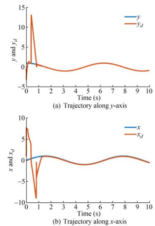 Figure 7 Tracking of the state response
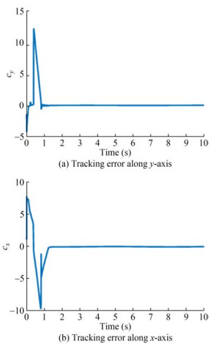 Figure 8 Tracking error
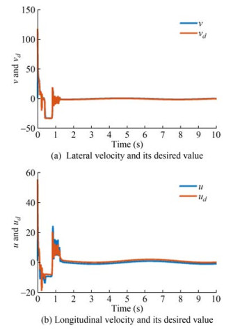 Figure 9 Tracking of the velocity variable
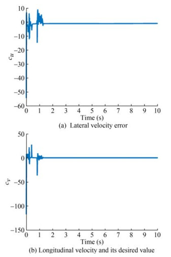 Figure 10 Velocity tracking errors
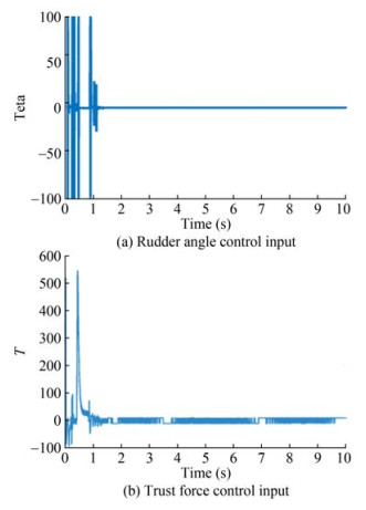 Figure 11 Control inputs
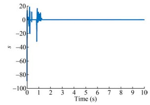 Figure 12 Sliding surface
Figure 7 displays both the state variables, their convergence to the desired value in a finite time. Time responses of the tracking errors are exhibited in Figure 8. These can be shown fast convergence of the tracking errors to zero.
Using the proposed controller, the velocity tracking errors are presented in Figure 9.
Figure 10 displays the control inputs trajectories. The boundedness of all signals involved in the overall system are obvious.
The sliding surface is illustrated in Figure 12. As it can be shown, sliding surface converges to zero in limited time.
Comparing the proposed exploration with that of (SiraRamírez, 2002) and based on Figures 7-13, the proposed technique 1 - has the faster convergence to zero, 2 - is robust against external disturbance.
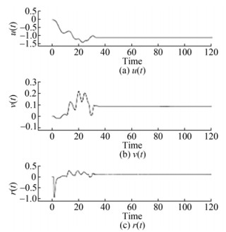 Figure 13 Velocity variable (Sira-Ramírez, 2002)
As shown in above figures, this technique guarantees 1) the robustness against disturbances and uncertainties, 2) the tracking of desired trajectory, 3) the chattering phenomena reduction and 4) stability of closed loop system.
6 Conclusion
This article deals with a super-twisting sliding mode control design for a class of nonlinear FO chaotic systems and a terminal sliding mode control design for Hovercraft. To illustrate the closed-loop system's stability, theoretical analysis has been provided by candidate Lyapunov function. Robustness of the suggested controller in the presence of the external disturbances and the convergence of tracking error to origin are the chief advantages of the suggested controller design procedure. The promising functionality of the mentioned procedure is confirmed according to the simulation results. The systems represent excellent performance and fine effectiveness. Future studies can be done to control fractional-order uncertain chaotic systems using adaptive sliding mode, control laws and intelligent network.
Competing interestThe authors have no competing interests to declare that are relevant to the content of this article. -
Figure 1 Outline of hovercraft model
Figure 2 Original system's state variable
Figure 3 Proposed method's state variable with $[x(0), y(0), z(0)]=$ $[9, 1, 9]$
Figure 4 The proposed sliding surface trajectory
Figure 5 Proposed control input
Figure 6 State variable (Aghababa, 2013)
Figure 7 Tracking of the state response
Figure 8 Tracking error
Figure 9 Tracking of the velocity variable
Figure 10 Velocity tracking errors
Figure 11 Control inputs
Figure 12 Sliding surface
Figure 13 Velocity variable (Sira-Ramírez, 2002)
Table 1 The symbols of hovercraft dynamics
Symbol Explanation $ a $ The arm length from mass center to the surface of rudder $ v $ Lateral velocity $ r $ Angular velocity $ \theta $ Rudder angle $ T $ Trust force $\left\{u_d, v_d, x_d, y_d\right\}$ Desired parameters $\left\{d_{u_0}, d_{v_0}, d_{r_0}, d_u, d_v, d_r\right\}$ Friction coefficients $ m $ Mass of hovercraft $ J $ Inertia moment $ u $ Longitudinal velocity $\left[\begin{array}{cc} \cos \theta & \sin \theta \\ -\sin \theta & \cos \theta \end{array}\right]$ Rotational matrix (ex, ey) Position tracking errors (eu, ev) Velocity errors bT Force scaling coefficient -
Aghababa MP (2013) Design of a chatter-free terminal sliding mode controller for nonlinear fractional-order dynamical systems. International Journal of Control 86(10): 1744–1756. https://doi.org/10.1080/00207179.2013.796068 Alipour M, Malekzadeh M, Ariaei A (2022) Practical fractional-order nonsingular terminal sliding mode control of spacecraft. ISA Transactions 128(4): 162–173. https://doi.org/10.1016/j.isatra.2021.10.022 Aslam MS, Raja MAZ (2015) A new adaptive strategy to improve online secondary path modeling in active noise control systems using fractional. Signal Processing Approach 107: 433–443. https://doi.org/10.1016/j.sigpro.2014.04.012. Cabecinhas D, Batista P, Oliveira P, Silvestre C (2017) Hovercraft control with dynamic parameters identification. IEEE Transactions on Control Systems Technology 26(3): 785–796. https://doi.org/10.1109/TCST.2017.2692733 Couceiro MS, Ferreira NF, Machado JT (2010) Application of fractional algorithms in the control of a robotic bird. Communications in Nonlinear Science and Numerical Simulation 15(4): 1–11. https://doi.org/10.1016/j.cnsns.2009.05.020 Djeghali N, Bettaye M, Djennoune S (2021) Sliding mode active disturbance rejection control for uncertain nonlinear fractional-order systems. European Journal of Control 57(1): 54–67. https://doi.org/10.1016/j.ejcon.2020.03.008 Hu R, Deng H, Zhang Y (2020) Novel dynamic-sliding-mode-manifold-based continuous fractional-order nonsingular terminal sliding mode control for a class of second-order nonlinear systems. IEEE Access 8: 20–29. https://doi.org/10.1109/ACCESS.2020.2968558 Jeong S, Chwa D (2017) Coupled multiple sliding-mode control for robust trajectory tracking of hovercraft with external disturbances. IEEE Trans Ind Electron 65(5): 4103–4113. https://doi.org/10.1109/TIE.2017.2774772 Karami H, Ghasemi R (2020) Fixed time terminal sliding mode trajectory tracking design for a class of nonlinear dynamical model of air cushion vehicle. SN Applied Sciences 2: 98. https://doi.org/10.1007/s42452-019-1866-5 Levantovsky LV, Levant A (1987) High order sliding modes and their application for controlling uncertain processes. Moscow: Institute for System Studies of the USSR Academy of Science 18: 381–384 Li R, Zhang X (2022) Adaptive sliding mode observer design for a class of T–S fuzzy descriptor fractional order systems. IEEE Transactions on Fuzzy Systems 28(9): 1951–1960. https://doi.org/10.1109/TFUZZ.2019.2928511 Li Y, Chen YQ, Podlubny I (2009) Mittag-Leffler stability of fractional-order non-linear dynamic systems. Automatica 45(8): 1965–1969. https://doi.org/10.1016/j.automatica.2009.04.003 Lorenz EN (1963) Deterministic non-periodic flow. Journal of the Atmospheric Sciences 20: 130–141. https://doi.org/10.1175/1520-0469(1963)020<0130:DNF>2.0.CO;2 https://doi.org/10.1175/1520-0469(1963)020<0130:DNF>2.0.CO;2 Magin RL (2006) Fractional calculus in bioengineering. Begell House Redding Modiri A, Mobayen S (2020) Adaptive terminal sliding mode control scheme for synchronization of fractional-order uncertain chaotic systems. ISA Transactions 105(1): 33–50. https://doi.org/10.1016/j.isatra.2020.05.039 Munoz E, Gaviria C, Vivas A (2007) Terminal sliding mode control for a SCARAR robot. International Conference on Control, Instrumentation and Mechatronics Engineering, Johor Bahru, Johor, Malaysia Ott E, Grebogi C, Yorke J (1990) Controlling chaos. Physical Review Letter 64(11): 1196–1199. https://doi.org/10.1103/PhysRevLett.64.1196 Petras I (2010) Fractional-order nonlinear systems-modeling, analysis, and simulation. Spring-Verlag, Berlin Podlubny I (1998) Fractional differential equations: An introduction to fractional derivatives, fractional differential equations, to methods of their solution and some of their applications. Academic Press, 198 Rabah K, Ladaci S, Lashab M (2017) A novel fractional sliding mode control configuration for synchronizing disturbed fractional-order chaotic systems. Pramana - J Phys 89(46): 1443–1447. https://doi.org/10.1007/s12043-017-1443-7 Rook S, Ghasemi R (2018) Fuzzy fractional sliding mode observer design for a class of nonlinear dynamics of the cancer disease. International Journal of Automation and Control 12(1): 62–77. https://doi.org/10.1504/IJAAC.2018.10005623 Shahbazi F, Ghasemi R, Mahmoodi M (2021) Fractional nonsingular terminal sliding mode controller design for the special class of nonlinear fractional-order chaotic systems. International Journal of Smart Electrical Engineering 11(2): 83–88. https://doi.org/10.30495/ijsee.2022.1945459.1160 Sharafian A, Ghasemi R (2019) A novel terminal sliding mode observer with RBF neural network for a class of nonlinear systems. International Journal of Systems, Control and Communications 9(4): 369–385. https://doi.org/10.1504/IJSCC.2018.10012813 Sharafian A, Ghasemi R (2019) Fractional neural observer design for a class of nonlinear fractional chaotic systems. Neural Computing and Applications 31(4): 1201–1213. https://doi.org/10.1007/s00521-017-3153-y Sira-Ramírez H (2002) Dynamic second-order sliding mode control of the hovercraft vessel. IEEE Transactions on Control Systems Technology 10(6): 860–865. https://doi.org/10.1109/TCST.2002.804134. Song S, Zhang B, Xia J, Zhang Z (2018) Adaptive back stepping hybrid fuzzy sliding mode control for uncertain fractional-order nonlinear systems based on finite-time scheme. IEEE Transactions on Systems, Man, and Cybernetics: Systems 20(4): 1559–1569. https://doi.org/10.1109/TSMC.2018.2877042 Tavazoei MS, Haeri M, Jafari S, Bolouki S, Siami M (2008) Some applications of fractional calculus in suppression of chaotic oscillations. IEEE Transactions on Industrial Electronics 55(11): 4094–4101. https://doi.org/10.1109/TIE.2008.925774 Utkin V (1992) Sliding mode in control and optimization. Springer Verlag, Berlin Wang N, Gao Y, Zhang X (2021) Data-driven performance-prescribed reinforcement learning control of an unmanned surface vehicle. IEEE Transactions on Neural Networks and Learning Systems 32(12): 5456–5467. https://doi.org/10.1109/TNNLS.2021.3056444 Wang N, Su SF (2019) Finite-time unknown observer-based interactive trajectory tracking control of asymmetric under actuated surface vehicles. IEEE Transactions on Control Systems Technology 29(2): 794–803. https://doi.org/10.1109/TCST.2019.2955657 Xu H, Fossen TI, Guedes Soares C (2020) Uniformly semiglobally exponential stability of vector field guidance law and autopilot for path-following. European Journal of Control 53(1): 88–97. https://doi.org/10.1016/j.ejcon.2019.09.007 Xu H, Oliveira P, Guedes Soares C (2021) L1 adaptive back stepping control for path-following of under actuated marine surface ships. European Journal of Control 58(1): 357–372. https://doi.org/10.1016/j.ejcon.2020.08.003