1   Introduction

For a long time, many scholars and engineers have carried out extensive research on drag reduction and cavities. Underwater vehicles are developing in the direction of long sailing distances, high speed, and intelligence (Ashley, 2001; Savchenko, 2001). To consider a vehicle's index of long sailing distance and high speed, researchers usually optimize the design to meet the requirements. The supercavitating technology represents a successful result of such optimization. Supercavitating vehicles use a special hydrodynamic layout, which makes full use of supercavity features. The drag is greatly reduced as if flying in the air. The kinetic energy supercavitating projectile is efficient in drag reduce. It has a high or ultra-high speed and can achieve precise and fast damage for targets in water.

The former Soviet Union used cavitation to increase the torpedo velocity to nearly 100 m/s (Zhang et al., 2014). This supercavity drag reduction technology is a milestone for underwater vehicles. However, the single-phase flow becomes a multi-phase flow, which has many disturbance factors and is difficult to analyze and calculate in theory (Wei et al., 2013). When a vehicle moves with supercavity, most of the forces that act on it will disappear. The force of the vehicle becomes highly nonlinear, which often leads to deflection and loss of control. These difficulties are an unprecedented challenge for mathematical modeling and stability research of vehicles (Ruzzene and Soranna, 2004; Zhang et al., 2010; Wei et al., 2012; He et al., 2013; Mirzaei et al., 2015).

The stability analysis method mainly uses mathematical modeling or experiments. The experiments of kinetic energy supercavitating vehicles usually require substantial human and financial resources, which is inconvenient.

Theoretical modeling is highly imperative to determine a vehicle's motion features. The model can reveal the mechanism of a vehicle's motion in theory. Rand et al. (1997) proposed the simplistic supercavitating vehicle model, which mainly focuses on the frequency of tail slaps. The body coordinate origin is located at the cavitator, and it supposes that the vehicle rotates around the cavitator on the plane. The results indicate that the frequency of tail slaps will decrease as speed decreases. In addition, the frequency of tail slaps highly depends on the initial condition. Richard Rand's model is great in simplification, and it is deemed instructive for the later supercavitating vehicle research. He et al. (2013) combined Richard Rand's theory and finite element method (FEM) and established a procedure for supercavitating vehicles. The results revealed not only the dynamic features but also the loads of tail slaps. The findings also highly accorded with those of Richard Rand. Zhao et al. (2018, 2019) proposed the hypothesis of mirror tail slap, which is a tail slap model based on Richard Rand's work. The tail slaps were simulated in the cavity cross section at the vehicle's tail position. The results also showed the trajectory of this vehicle. This previous work is preliminary research for stability.

The above works were based on Richard Rand's theory. However, Richard Rand's model is based on the single degree of freedom (DOF) vibration theory. A limitation of this model is that it cannot reveal the mechanism of stability in depth.

Therefore, Kulkarni and Pratap (2000) proposed a 3DOF model in the longitudinal plane as early as 2000. In this model, the motions of tail slaps and those in supercavity are considered separately. In addition, the model is highly nonlinear, which was verified by the computational fluid dynamics (CFD) method. Two kinds of vehicles are simulated by this model. The results indicated that although tail slapping occurred, the trajectory of the vehicle remained linear. This work also proposed an equation about the tail slap angular velocity. Their proposed model is the foundation of many works on stability. To gain a qualitative understanding of stability, Savchenko (2001) proposed four criteria for judging the stability of supercavitating vehicles. These criteria covered the velocity from 50 to 1 000 m/s, which was based on numerous experimental results, and included double-cavity, sliding, tail slapping, and aerodynamic-hydrodynamic stabilities. Savchenko's results were very institutive for future works. Sail S. Kulkarni and Savchenko provided pioneering works for the study of stability.

The 3DOF dynamic model of Sail S. Kulkarni is considerably better than Richard Rand's work. However, this 3DOF model excludes the influence of attack angle. Zhou et al. (2016) added the influence of attack angle and many uncertainty influences during motion. Moreover, the uncertainty of trajectory was analyzed based on these works. The results were verified by experiments in the literature. This previous work was considered instructive for engineering. Nguyen Thai et al. (2018) established an accurate 3DOF model and evaluated it by experiment. This model is based on exterior ballistics, and it is more scientific compared with previously proposed models. The error was nearly 1.1%. Their work verified for the first time a mathematical model using experiments. Wang et al. (2020) proposed a 6DOF model for kinetic supercavitating vehicles. This model was verified by three kinds of vehicles. In addition, the dynamic features were explored and showed a special dynamic behavior in space. Finally, a new stability evaluation method was proposed, and it was meaningful for theoretical supercavitating research.

Multiple analysis methods have been proposed for years. As a result, the 6DOF dynamics model is more useful than others in exploring the features of kinetics and dynamics and can be used to analyze the mechanism of instability in theory. For kinetic energy supercavitating vehicles, the stability is influenced by the vehicle structure, hydrodynamic environment, and initial conditions. A fluctuating initial condition in a small sailing distance has a minimal impact on stability unless other unpredictable disturbances occur when the vehicle is launched. These factors directly determine whether the target can be destroyed. The vehicle's structure is the most important factor affecting its performance. On the other hand, stability is a key index to measuring the hydrodynamic layout of supercavitating vehicles and is the basis of the following studies. However, quantitative analysis of vehicle stability in the past was difficult. The stability of supercavitating vehicles by experiments is very inconvenient and costs a huge amount of manpower, material, and financial resources.

Most scholars believe that large supercavitating vehicles (LSVs) and small supercavitating vehicles (SSVs or projectiles) have the same dynamic model or behavior. However, the dynamic behavior and model were dramatically different from recent experiments on water. These test data were from authors' previous works and relative literature. From the tail slap angular velocity view, the angular velocity of SSVs is ten times more than that of LSVs. The difference was considered in depth. The established dynamic model also differed. For instance, the supercavity calculation strategy must consider the physical dimension. The memory effect and cavity drift features are considered imperative for LSVs but not for SSVs. These differences will make the dynamic models diverse, which leads to different optimization strategies. The early optimization problem mainly focuses on cavitators because they are important for supercavity configuration. Scholars have conducted many works on the cavitator area, and the research methods used varied. Choi et al. (2005) used the potential theory to optimize the cavitator to minimize the drag, and the cavity shape was calculated. The author's work is based on a gradient optimization algorithm, which can simultaneously optimize the cavitator and cavity. Jiang et al. (2009) converted the free-boundary value problem of supercavities into an equivalent shape optimal problem. The objection function was defined by the integral square error of pressure difference. Then, the optimization of the cavitator and cavity boundary calculation were merged into a multi-objective optimization problem. However, the author designed the cavitator without considering the vehicle's structure layout. Ahn et al. (2010) optimized an LSV with a control system that included configuration, mass distribution, and manipulator. A limitation of this work was the vehicle velocity (170–200 m/s). Shafaghat et al. (2011) defined a multi-objective optimization problem to optimize the cavitator shape. Based on the flow characteristic and cavitator model, the design parameters and constraint conditions were obtained. Then, Non-dominated Sorting Genetic Algorithms-Ⅱ was employed to optimize this issue. The results were compared with those of the classical optimal method, which showed that the cone-shaped cavitator was optimal in the current condition. Mirzaei and Taghvaei (2019) optimized the configuration of a ventilated supercavitating vehicle. The layout was compared between a natural supercavitating vehicle and its ventilated counterpart. The results showed that the ventilated case had a smaller cavity radius than the natural one. The supercavitating vehicle design is aimed at the cavitator structure. The method is mainly based on potential theory and CFD. The dynamic method is rarely used. In addition, some researchers combined the optimal algorithm with FEM, which involves complicated computations; thus, the method is inconvenient to use in engineering.

In our previous work (Wang et al., 2020), we put forward the quantitative criterion for the stability of supercavitating projectiles, and it can be used to predict a projectile's motion by the numerical method. Thus, the hydrodynamic layout of this projectile can be changed quickly, and the resources can be saved. In this work, we mainly focused on solving the optimization problem of high-speed projectiles. A complete program about the projectile's optimal condition, which is also based on genetic algorithm (GA), was explored. The program has a good generality and can meet the accuracy of engineering. An optimal hydrodynamic layout was obtained by the 6DOF model based on the improved GA. For guiding the engineering design, the dynamic features of this optimized projectile were analyzed by the 6DOF model. The results showed that this projectile has a self-stability tendency, which is a special motion. The self-stability tendency is closest to the ideal motion and the optimal design results. This structure is instructive for the design of kinetic energy supercavitating projectile.

2   Mathematical model of supercavitating projectiles

A complete mathematical model was proposed in Wang et al. (2020). Therefore, all the reference coordinate system definitions, coordinate transformation, parameters, and formulation derivation can be referred to in Wang et al. (2020). This work is a continuation of previous work. The supercavitating projectile's research needs not only experiments but also a mathematical model. The quantitative description of the projectile's velocity and attitude is important to study the various phenomena during motion, and the model can reveal the dynamic features in nature. In addition, a reasonable model is required for further research about the projectile's motion. To simplify this model, we analyzed the body coordinate system (Ox₁y₁z₁). The motion equations are listed as follows:

a. Dynamic equations:

b. Kinetic equations:

c. Geometric equations:

d. Supercavity equations:

e. Hydrodynamics coefficient equations:

f. Angle equations:

g. Motion converting equations:

Eqs. (1)–(18) show the scalar equations used to describe the motion of supercavitating projectiles. These equations are strongly nonlinear and ordinary differential equations. In the process of establishing the above equations, given the limitations of the problems studied, the applicable range of velocity was between 100 and 900 m/s. Moreover, considering the low gas density in the supercavity, the aerodynamic force of the projectile in the cavity was ignored. The motion equation was continued by a hyperbolic function for the convenience of analysis.

Wang et al. (2020) validated the 6DOF model using four methods.

In the first verification case, we employed an experiment on kinetic energy supercavitating projectiles. The supercavity model was validated by the test data. The maximum test sailing distance served as a preliminary validation for this model.

In the second verification case, we compared the model results with those of the classical model, which is a single DOF model. The 6DOF supercavitating model is a precise model that considers many factors. However, the classical model only considers the drag of the cavitator. The displacement of the 6DOF model is less than that of the classical model's counterpart in theory. The 6DOF model greatly rectifies the classical model. Their velocity curves have high similarity. Therefore, the 6DOF model correctly predicts the projectile's motion underwater.

In the third and fourth verification cases, we used two groups test results and projectile data recorded in Zhao et al. (2014) and Nguyen Thai et al. (2018). The results of the test and numerical calculation were consistent, which proves the accuracy of the 6DOF model.

3   Stability of supercavitating projectile

3.1   Stability criterion

The stability of the kinetic energy supercavitating projectile is a key factor in evaluating its ballistics capability. Quantitative research is a significant method for the stability of supercavitating projectiles. When h_ef is equal to 0, tail slapping occurs exactly. Therefore, the limitation angle of tail slaps χ_lim is defined as follows (Wang et al., 2020):

The limitation angle of tail slaps χ_lim reflects the relative position of the projectile and the supercavity at the projectile's tail location. When χ, which is the angle between the supercavitating body axis and the horizontal line that passes through the mass center, is greater than the χ_lim, tail slaps will occur, and vice versa. Therefore, depicting χ and χ_lim on the same figure is meaningful. The χ−χ_lim curve has the following features (Figure 1):

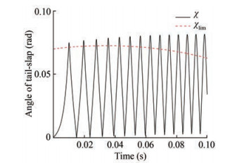Figure  1  χ−χ_lim curve (Wang et al., 2020)

Download: Full-Size Img

1) The χ−χ_lim curve can reflect the stability of the supercavitating projectile. If the projectile has stability with tail slaps, then the χ curve will sustain oscillation and pass through the χ_lim curve.

2) The χ_lim was used for the boundary. The proportion of χ below or above the χ_lim reflects the degree of motion stability.

When the upper part of χ, which is above χ_lim, is greater than the counterpart below, serious tail slaps of the projectile occur. This finding indicates that the projectile's body wetting would increase, and the drag is also increase. These factors will enhance the rate of attitude, reduce the displacement, and deflect the trajectory. In other words, the stability is relatively poor. However, when χ is totally above χ_lim, the supercavity cannot reduce the drag, and the projectile loses its stability. However, when the χ is under χ_lim completely, the projectile moves into the supercavity without making contact with it, which is an ideal state for supercavitating projectile. Thus, the projectile can balance the force and moment simultaneously due to the attack angle change.

3.2   Ideal stability for supercavitating projectile

Savchenko (2001) believes that the motion of a supercavitating projectile in the cavity varies with speed. Three cavitation schemes can be considered (v < 70 m/s): the stable sliding along the inner surface of the cavity (v = 100–200 m/s), mutual impact with the cavity wall (v < 900 m/s), and aerodynamic interaction with the cavitating steam splashing medium (v > 1 000 m/s). Four different stability mechanisms occur in turn. Theoretically, the ideal motion mode of a supercavitating projectile is the complete movement of the projectile into the cavity during motion. The definition of self-stability is introduced here as follows:

Self-stability: In the underwater motion of a supercavitating projectile, only the cavitator is in contact with water, and the rest is completely in the supercavity.

Section 3.1 presents a special motion mode of supercavitating projectile. In this case, the kinetic energy supercavitating projectile has self-stability. However, the ideal motion is hard to achieve due to the unpredictable disturbance in water, which is mainly caused by turbulence flow and many uncertainty factors.

According to the definition of self-stability, a mathematical model can be established for qualitative analysis. If the ideal self-stability exists, the relation is held as follows:

Substituting the definition of χ and χ_lim into Eq. (20), we have the following:

Simplifying Eq. (21), we attain the following equation:

Substituting the supercavity equation into Eq. (22), we attain the following:

Meanwhile, the self-stability equation also holds:

The angular velocity ω_x1 = 0 rad/s and roll angle θ = 0 rad are used in Eqs. (24)–(28), which are constrained by the cavitation number σ(t), pitch angle ψ, and yaw angle φ. The relation between the parameters of Eq. (23) is extremely complicated and strictly defined in mathematics. Meanwhile, the numerical results indicated that the solution is always divergent under a small initial disturbance.

This conclusion was also obtained by the following optimization results. Therefore, designing a kinetic energy supercavitating projectile to keep an ideal self-stability when the projectile moves in water is impossible (the velocity is between 300 and 900 m/s). If the projectile achieves selfstability, then the control strategy must be employed in this projectile, which can cause hydrodynamic forces to constantly shift positions to balance the gravity and disturbances of the projectile.

3.3   Optimizing the projectile's structure

For the above features, the χ−χ_lim curve is a key basis for judging the stability of a supercavitating projectile. Figure 1 shows the χ−χ_lim curve based on the conditions in Table 1. The curve indicates that this projectile can achieve stable motion under this structure (Figure 2) and the initial conditions.

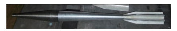Figure  2  Structure of supercavitating projectile (Wang et al., 2018a)

Download: Full-Size Img

However, the proportion of the χ above χ_lim gradually increased with the projectile motion. This condition Eq. (20) suggests the increasingly serious strengthening of the tail slaps. Tail slapping is an important factor in velocity attenuation. The calculation results showed that the displacement of this projectile was 25 m. Although this supercavitating projectile was stable, its sailing distance was short and could not meet the design requirements. Therefore, a reasonable structure design is imperative.

4   Optimization of the structure of supercavitating projectiles

The stability of supercavitating projectiles is affected by many factors, which include initial disturbances, motion disturbances, flow velocity, and fluid structure. The initial disturbances, motion disturbances, and flow velocity are external factors, and the fluid structure is an internal factor. From mathematical point of view, the projectile's configuration is the parameter of dynamic system, which determines the evolution direction of the nonlinear dynamic system. Therefore, the projectile's structure is significant for stability. The design objective meets the design requirements, which allows the projectile to achieve exceptional sailing distance and damage effect.

4.1   Simplification of the projectile structure and calculation

The supercavitating projectile's shape is complicated. Mechanical parameters, such as the moment of inertia, mass, and volume, are usually obtained by the software SolidWorks. The complex structure parameters will increase the number of optimal objective functions. The number of objective functions will greatly increase the difficulty of optimization and reduce the solving speed. Meanwhile, when the supercavity totally covers the projectile, the local structure, such as the fin, which is the transition part between the fin and cylinder, has a minimal effect on the projectile's motion. One of the most notable problems is the fins. For kinetic supercavitating projectiles, the tail is not designed to generate aerodynamic force inside the cavity but to gain an amphibious property. The gas inside the supercavity is thin, and the aerodynamic force will not affect the motion of the supercavitating projectile under a non-hypervelocity condition (V < 900 m/s).

Kinetic energy supercavitating projectiles feature small volume and light mass. The action mode of tail slaps is essentially different from that of large supercavitating projectiles.

The cavity diameter of the tail of the kinetic supercavitating projectile is relatively large and approximately 2–3 times larger than the projectile's tail diameter. In this paper, the cavity diameter was around 2.3 times larger and completely wrapped the projectile. When tail slaps occur, its tail is in unilateral wet. Given the high speed of kinetic energy supercavitating projectiles, secondary cavitation usually occurs at the fin. Secondary cavities on different fins affect each other and merge. Such an effect is equivalent to that of treating the tail as a cylinder. In addition, given the small size of the supercavitating projectile, the secondary cavitation effect of the fin has minimal influence on the cavity during tail slaps. Figure 3 shows the test results of the fin (Wang et al., 2018b). The fin height H was 24 mm. Figure 3 also reveals the test results of the fin piercing cavities with diameters of 18, 12, and 6 mm. The influence of fin on the cavity is very significant in the cases of a and b but very weak in the case of c. In this work, the height of the fin H was 3.28 mm, and the influence on the cavity can be ignored. Therefore, the influence of the fin on the tail slap force was ignored.

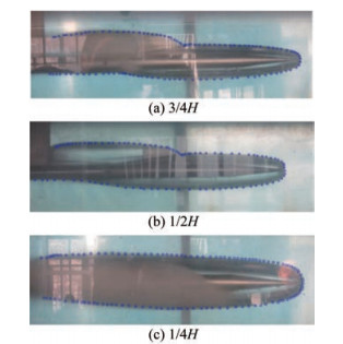Figure  3  Experiment results (Wang, 2018b)

Download: Full-Size Img

Most of the designs of kinetic energy supercavitating projectiles lack fins. Given that almost no aerodynamic stability mechanism is available for kinetic energy supercavitating projectiles when the flight speed is less than 1 000 m/s, the tails are non-functional underwter. The details can be found in Zhang et al. (2014).

However, large supercavitating projectiles are different. Large supercavitating projectiles have lower speeds than kinetic supercavitating projectiles and control and propulsion systems, and the cavity diameter of the projectile tail is usually 1.5–2 times that of the projectile tail. The deflection angle is generated by the fin's deflection, which can generate hydrodynamic force and control the attitude of the projectile. Therefore, the fins of supercavitating vehicles usually pierce the supercavity. Thus, the influence of the fins on supercavity cannot be ignored.

The large-scale and small supercavitating vehicles mainly involves the following three differences:

1) From the launch point of view, the launch of supercavitating vehicles mainly depends on the launcher and launch system. Its diameter is close to that of a missile or torpedo. However, supercavitating projectiles rely on high-density and high-speed small-caliber artillery and machine guns to launch.

2) From the perspective of motion mode, supercavitating vehicles are usually equipped with a control system with a navigation speed of 50–200 m/s, a large sailing distance, and a long navigation time. However, the supercavitating projectile has a sailing speed between 200–1 500 m/s; its motion completely depends on its own kinetic energy, and its sailing distance and sailing time are small.

3) From the perspective of the generation mechanism of supercavity, the supercavity generation of supercavitating vehicles mainly occurs through ventilation. By changing the ventilation and thermodynamic state of the gas, the shape of the supercavity is controlled to change the navigation state of the vehicle. However, supercavitating projectiles rely entirely on their cavitators to produce a supercavity. The change in their velocity will modify their supercavity morphology and eventually cause their gradual evolution toward instability.

A simplified structure was used to derive the formulation of mass center, mass, and moment of inertia. The formulation's result (I_x1=1.538×10⁻⁴ kg·m², I_z1=I_y1=1.436×10⁻⁶ kg·m², m=0.095 7 kg, x_cm=5.99×10⁻² m) is extremely close with that obtained by the software (I_x1=5.82×10⁻⁴ kg·m², I_z1=I_y1= 1.59×10⁻⁶ kg·m², m=0.116 kg, x_cm=6.025×10⁻² m). The mass center error was less than 1%. However, the resulting I_i1 (I_y1, I_z1) was relatively large. This outcome was caused by the simplification of calculations. The moment of inertia was mainly used to calculate attitude angles. However, the attitude angles change was small for the projectile with stable motion. Meanwhile, the order of magnitude of I_i1 (I_y1, I_z1) was consistent with those obtained with formulations and software. Thus, the moment of inertia could not make large errors. For I_x1, the fin stability method was employed in the amphibious supercavitating projectiles without a rotating stability. Therefore, I_x1 had a slight influence on this structure optimization problem. In summary, we ignored the local structures to accelerate the calculation and improve the efficiency of design. Figures 4 and 5 show the original and simplified structures, respectively.

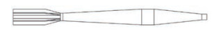Figure  4  Original structure (Wang et al., 2019)

Download: Full-Size Img

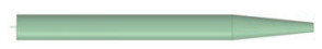Figure  5  Simplified structure

Download: Full-Size Img

The simplified structure has four parameters: the length of cylinder part L₁, diameter of cylinder part D, diameter of cavitator d, and length of frustum of cone L₂.

For optimal calculation, the formula of the mass center and moment of inertia must be derived based on the simplified model. We set the coordinate origin at the cavitator center. Figure 6 shows the projectile's axis, that is, the z axis. The material of frustum of cone L₂ was tungsten alloy (density: 18.75 g/cm³), and that of cylinder part L₁ was aluminum (density: 2.7 g/cm³). According to the coordinate of the cavitator, the mass center position of x and y were 0 and 0, respectively. The value of z can be calculated as follows:

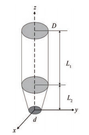Figure  6  Coordinate of cavitator

Download: Full-Size Img

Eq. (29) can be calculated in two steps as follows:

Step 1: Numerator:

Step 2: Denominator:

When the mass center was obtained by the above method, the coordinate origin moved to the mass center. The coordinate is called the principal axis system. The matrix of the moment of inertia degenerated to a diagonal matrix. According to the symmetry, the formulation I_y = I_x holds. The matrix of the moment of inertia was different due to the mass center position and needed to be divided into two cases for the analysis:

When z₀ > L₂ holds, the mass center is located on the cylinder part, and the moment of inertia I_x can be calculated as follows (Figure 7):

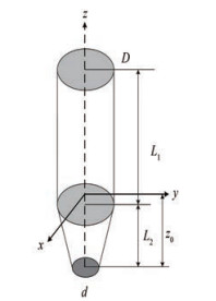Figure  7  Coordinate of mass center on the cylinder part

Download: Full-Size Img

When z₀ < L₂ holds, the mass center is located on the frustum of the cone part, and the moment of inertia I_x can be calculated as follows (Figure 8):

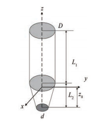Figure  8  Coordinate of mass center on the frustum of the cone part

Download: Full-Size Img

According to the parallel axis theorem, the coordinates of the mass center are the principal axes, and therefore, the moment of inertia I_z is constant. The formulation is as follows:

4.2   Optimization of algorithm design

Holland (1992) researched the GA theory and method. GA is a highly parallel, random, and self-adaptive algorithm developed from the mechanism of natural selection and evolution in biology. In short, it uses the population to search for optimal solutions, and the population represents a group of solutions. By applying a series of genetic operations, such as selection, crossover, and mutation, to the current population, a new generation is generated, and the population gradually evolves to contain an approximate optimal solution. This optimal solution is not accurate in mathematics, but the approximate solution meets the basic design requirements (Vaissier et al., 2019; Chan et al., 2020; Costa-Carrapiço et al., 2020; Ramos-Figueroa et al., 2020; Wang and Sobey, 2020).

Therefore, in this section, the approximate optimal solution was found based on the GA (Vaissier et al., 2019), and the algorithm was improved to optimize the offline projectile. The improved algorithm can be applied well to the optimization of projectile parameters, and it can accelerate the calculation speed.

For the optimization of this design problem, an optimization problem with a clear mathematical equation must be constructed first. Thus, the time series {t_n}, which is the time corresponding to the intersection point between χ and χ_lim, was introduced. This time series is important for stability analysis. If the time series {t_n} is long, the frequency of tail slap is high. A high tail slap frequency is disadvantageous to the projectile's stability and can increase the drag of flight. During the design of a supercavitating projectile, the number of tail slaps should be minimized as much as possible. The maximum of the time series {t_n} reflects the stable flight distance of the supercavitating projectile. When this projectile flight is 0.1 s, the maximum {t_n} is close to 0.1 s, which indicates that the projectile can fly stably for a long time. This condition can be written as follows:

where k_p is the scale factor between 0 and 1 and t_p is the time of this projectile's movement.

If the projectile has minimized tail slap number and long sailing distance, its structural design is optimized. Therefore, {t_n} can be one of the constraint conditions, and the sailing distance can be the objective function of this optimization issue. The projectile's sailing distance and the number of {t_n} restrict each other. The most important concern in the design is the sailing distance. If the design sailing distance can be reached, then the number of {t_n} is not important for engineering.

In summary, this optimization problem can be written as follows:

4.2.1   Note for initialization of the population

Traditionally, the initial individuals of the population, which are single variables, are generated randomly in a certain range. Four variables were considered parameters of the projectile structure in this work. These parameters feature synergies and control the motion of the projectile. The individuals of the population are the structural parameters and have four genes (cylinder length L₁, diameter of cylinder part D, diameter of cavitator d, and length of frustum of cone L₂). To ensure that good genes can be inherited between individuals during genetic operation, we assessed the stability of all generated individuals. The stability criterion was based on the maximum value of {t_n}. Supposing that the projectile's moving time is t_p, the maximum of {t_n} is {t_n}_max, and k_p is a coefficient between 0 and 1. If k_pt_p < {t_n}_max holds, then the projectile's motion is stable, and vice versa. When an individual is unstable, it needs to be regenerated and judged again until the initial population becomes stable and is outputted for use.

4.2.2   Note for fitness of the population

A range is used for the fitness evaluation of the population, and the fitness of the initial population is stored. In the first iteration, fitness can be used directly to avoid repeated calculations. For engineering, all individuals do not need to reach convergence completely; that is, the difference between individuals is less than 1%. Such accuracy is not significant for practice. Thus, after its calculation, the fitness must be evaluated to determine whether it can meet the engineering requirements. The fitness was evaluated by its mean value, and the difference vector between fitness and its mean value was solved. If the difference is acceptable, the final optimal results can be outputted.

4.2.3   Note for the initial condition of 6DOF dynamic equations

The initial value is the key to trajectory evolution. Therefore, the influence of the initial value of the 6DOF dynamic equations needs to be considered in the optimization problem to ensure that the optimized projectile can meet the requirements of trajectory dispersion, stability, and sailing distance under the small disturbance of the initial value. The projectile needs a certain generalization capability toward the initial value. Intermediate ballistics is a subject that studies the disturbance law of muzzle flow field to projectiles and mainly focuses on the disturbance phenomenon in the air (Li et al., 2015). In addition, the bore damage of the barrel has an important impact on its exterior ballistics (Shen et al., 2020a, 2020b). These two methods have become important in the study of the initial random disturbance of modern exterior ballistics.

These methods are also based on emission dynamics and the CFD method, but their calculation is large and complex, which is not conducive to engineering applications. Therefore, Monte Carlo simulation is still the main research method in modern external ballistics. In this work, ψ and φ were between − 0.05 and 0.05 rad. The ω_y and ω_z were between −1 and 1 rad/s.

The projectile was launched by a smooth-bore gun. Thus, ω_x = 0 rad/s and θ = 0 rad.

4.3   Basic flow of the algorithm

The traditional GA was improved to accelerate the calculation speed. Figure 9 shows the flow of this algorithm. The main structure of this algorithm is as follows:

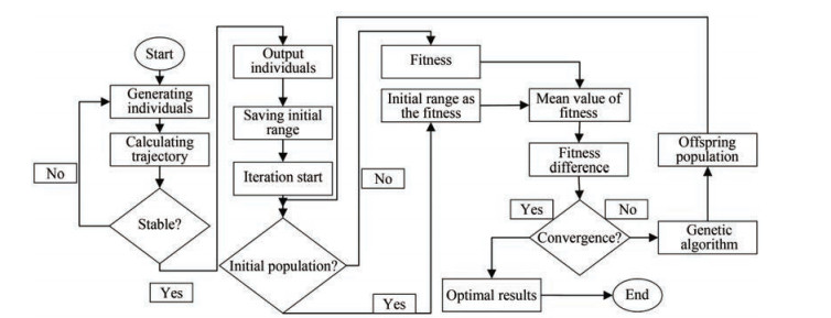Figure  9  Flow of GA improvement

Download: Full-Size Img

5   Dynamic features of the optimized projectile

5.1   Optimized results

For the maximum use of the initial kinetic energy of the projectile, the maximum sailing distance and stability should be achieved under the initial velocity. The maximum length of the projectile was not more than 200 mm, and the minimum length was not less than 100 mm. Given that the long rod projectile is beneficial for damaging the target, the slenderness ratio of the long rod projectile is generally greater than 10. The projectile's body consists of two materials: the frustum of the cone is tungsten alloy (density: 18.75 g/cm³), and the cylinder part is aluminum (density: 2.7 g/cm³). The lengths of the frustum of the cone and the cylinder were between 50 and 100 mm. A 30 mm-caliber gun was used to launch the projectile. Considering the sabot design, the cylinder diameter cannot be adjusted in a large range. Therefore, the cylinder diameter was set in the range of [12.5, 12.56] mm, and that of the cavitator was [1, 12.5] mm. To ensure accuracy, we used a 22-bit binary code for coding. The initial population was 200, and 500 generations were set in the evolution. The cross probability was 0.7, the selection probability was 0.5, and the mutation probability was 0.001 for a general GA.

Table 2 shows the optimized projectile parameters. It meets the convergence requirements when it evolves to the 49^th generation. The projectile can have a large displacement. For the original structure, when the projectile moved for 0.1 s, its velocity was attenuated to 200 m/s. It reached the termination of this code because the code set 0.1 s as the motion time. However, the improved structure was different. When the projectile flight lasted for 0.1 s, the rest velocity was 437.84 m/s. The change in velocity was 62.16 m/s after 0.1 s. Currently, the rest velocity is considerable, and it not only has a strong penetration capability but can also increase the sailing distance. Therefore, the optimized projectile has a better water ballistic performance. The water ballistic performance is mainly evaluated by displacement. For a certain projectile, if the velocity decreases slowly, then the number of tail slaps is lessened, and a good tendency of self-stability is observed. Thus, the projectile is well designed. This projectile structure is instructive for the design of underwater projectiles with a large sailing distance. Therefore, the nature of stability, which is meaningful for engineering design, must be researched in depth. Figure 10 shows the optimized supercavitating projectile configuration and the conceptual design of amphibious supercavitating projectile. This optimized projectile features a large cone part, which has been found in Yi et al. (2008a, 2008b, 2008c, 2009a, 2009b). Meanwhile, the accuracy of this optimization procedure has also been verified. We provided the supercavitating projectile with a tail to inspire more scholars to further carry out the overall design research of amphibious supercavitating projectiles. The amphibious supercavitating projectile will become an important development direction of underwater ammunition in the future.

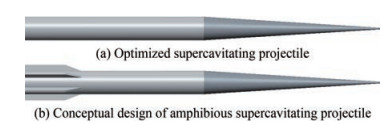Figure  10  Optimized configuration

Download: Full-Size Img

5.2   Mechanism of stability

Table 3 lists the calculation parameters. However, the matrix of the moment of inertia, mass center position, mass, and projectile length can be obtained by calculating the structural parameters. Thus, this optimized projectile is different from the original structure.

By the initial conditions in Table 2, the trajectory and attitude of the projectile can be calculated. First, for the kinetic energy supercavitating projectile, the most important thing is its stability. The good performance of the supercavitating projectile is based on a well-structured design. It is instructive for the projectile's design in future works. Therefore, the first task is to deeply explore the stability mechanism of this projectile. In our previous work, we proposed the χ−χ_lim curve to judge the stability. Figure 11 shows the χ−χ_lim curve of the optimized projectile. According to the stability criterion, the number of tail slaps was 8, which is beneficial for the projectile's stability. Thus, the projectile moved by 46.75 m. Meanwhile, when the χ−χ_lim curve was enlarged partly (Figure 12), the difference Δχ between χ and χ_lim curves was Δχ << 4×10⁻⁴ rad=0.017°. This result indicates that the supercavitating projectile belongs has a body-fitted cavity, which is close to the effect of film drag reduction theoretically. The findings also showed that when the tail slaps were about to occur, given its good self-stability, the tail slap motion did not proceed completely. Only the tail of the projectile touched the cavity, and the projectile showed the dynamic behavior of reverse rotation immediately. The tail slap action was largely weakened, and thus, the drag of this projectile can be reduced greatly. The results also revealed that the mathematical solution may be inconsistent with the dynamic behavior. Therefore, the stability criterion, which was proposed in our previous work, needs to be weakened. This relation can be written as follows:

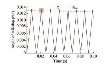Figure  11  χ−χ_lim curve

Download: Full-Size Img

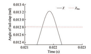Figure  12  Partly enlarged χ−χ_lim curve

Download: Full-Size Img

where {t_i} is maximum time array of χ, {χ_ti} and {χ_limti} are the function value of χ and χ_lim curves at {t_i}, respectively. ε is the weakening quantity. When all values of the sequence {χ_ti − χ_limti} are less than the ε, then the motion is weakened stability. The value of ε was set as 1°, that is, 0.017 45 rad.

The discussion above showed that self-stability only exists in theory. Notably, given the uncertainty of launch conditions and the environment, self-stability is difficult to maintain. The kinetic projectile approaches self-stability in a state of minimum energy consumption under current conditions, which is a universal law of nature, that is, the principle of minimum energy. For the actual needs, the weakened self-stability is defined as follows: the motion closest to self-stability.

In Section 3.2, we proposed the ideal motion equations of this projectile based on the stability criterion. Self-stability is a special motion that results in the complete projectile movement in the supercavity. In this condition, the best drag reduction effect can be achieved. This motion is impossible in theory because the gravity component in the vertical direction is hard to balance. Eqs. (24) – (28) represent an ideal case. However, in case of any disturbances, this ideal motion will be lost and transferred to the tail slaps.

Figure 11 shows a motion with a good self-stability tendency. This motion is an optimal one under the design. The experimental results also indicated that when the projectile's velocity was more than 1 000 m/s, that is, hypervelocity, the projectile approximately moved to the supercavity. However, the self-stability tendency, whose velocity is between 300 – 900 m/s, is different from the motion of hypervelocity. For the hypervelocity motion, the projectile will interact with the steam medium produced by the cavitation. The self-stability tendency is a projectile's inherent property. We have observed this phenomenon in experiments (Figure 13). The tail of the projectile first touched the smooth and stable supercavity, and then, the tail immediately left the wall and rotated in reverse. At this point, an instantaneous disturbance occurred on the supercavity, and a disturbance wave was generated on the supercavity and expanded continuously. The supercavitating projectile constantly moved in this mode within 0.1 s. Thus, the drag of the projectile was mainly the pressure difference drag, and the friction drag can be ignored during the tail slaps.

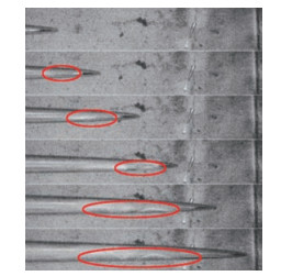Figure  13  Self-stability tendency

Download: Full-Size Img

Figure 13 displays the velocity curve of the projectile. A comparison of the results with the structure discussed in previous work (Wang et al., 2020) revealed the following characteristics:

1) Similarities: The mean value of kinetic energy dissipation in V_y1 and V_z1 directions was zero.

2) Differences: The velocity amplitude of the optimized structure in the direction of V_y1 and V_z1 was far less than that before optimization. This result suggests that the self-stability tendency of this projectile has less energy dissipation in V_y1 and V_z1 directions. The projectile's velocity attenuated slowly per second. Figure 14 also reveals the resultant velocity and velocity components V_x1 in x₁. The two curves are very close, which indicates that the attenuation of the projectile in the axial was consistent with the resultant velocity. The dissipation of kinetic energy was mainly used to overcome the pressure difference drag movement and increase the sailing distance.

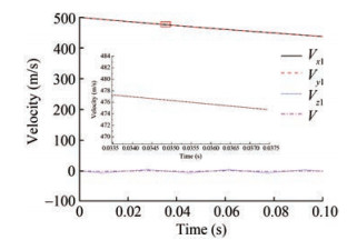Figure  14  Velocity curve

Download: Full-Size Img

Figure 15 shows the angular velocity curve. Compared with previous work, the angular velocity curve changed dramatically because of the projectile's good self-stability. When the projectile moved into the supercavity, the hydrodynamics acting on the cavitator consistently produced a restoring moment. The moment caused the projectile to rotate inversely. For the maintenance of stability, the hydrodynamics changed directions continually. This performance is related to the structural design. Moreover, although the angular velocity derivative was relatively large, the angular velocity was smaller than that of the projectile with poor stability. In addition, the angular velocity fluctuation range was between − 2.5 and 2.5 rad/s and stable during movement, which is also an important reason for projectile stable motion. Affected by the angular velocity, the pitch angle ψ, yaw angle φ, attack angle α, and sideslip angle β showed changes in a small range. The curve of the pitch angle ψ and yaw angle φ indicated that the behavior of this projectile was stable in water. The attack angle α, and sideslip angle β suggest that the body is less likely to overturn (Figures 16 and 17, respectively). These indicators all show the well-designed results of this projectile.

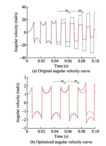Figure  15  Angular velocity before and after optimization

Download: Full-Size Img

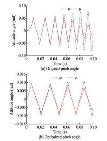Figure  16  Attitude angle before and after optimization

Download: Full-Size Img

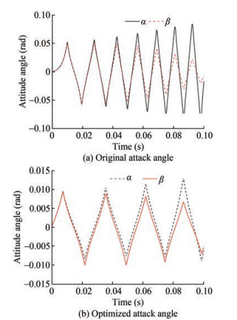Figure  17  Attack angle before and after optimization

Download: Full-Size Img

Figure 18 presents the displacement of the projectile. When the projectile moved by approximately 47 m in the x direction, the horizontal and vertical dispersions were 4.17 and less than 1 cm, respectively. Therefore, the self-stability tendency of projectile ballistic dispersion was also small. This feature is beneficial for the kinetic energy supercavitating projectile launched by a set number design. The projectile can impact the fixed target accurately in a short time for rapid damage in water.

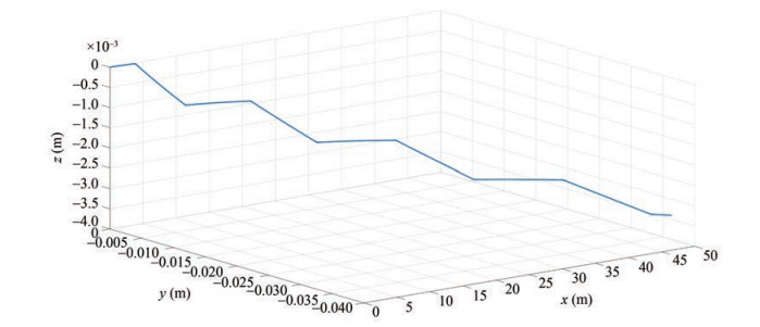Figure  18  Displacement within 0.1 s

Download: Full-Size Img

To fully show the advantages of the optimized projectile, we further provided the simulation results of the optimized projectile within 0.5 s here (Figure 19). Figure 19 shows that the optimized projectile had a sailing distance of nearly 200 m in 0.5 s and a residual speed of 291.4 m/s. Therefore, the optimized kinetic supercavitating projectile showed good performance in terms of the exterior and terminal ballistics.

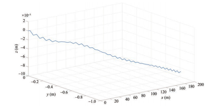Figure  19  Displacement within 0.5 s

Download: Full-Size Img

6   Conclusions

For kinetic energy supercavitating projectiles, stability and sailing distance are key factors in evaluating the projectile performance. These indicators are highly dependent on the structure. Therefore, the structure must have a reasonable design. To improve the sailing distance and stability of the supercavitating projectile, we optimized the projectile structure based on GA. The main conclusions are as follows:

1) Complete self-stability is difficult to achieve. Weakening self-stability is the closest motion state to self-stability in the actual process of supercavitating projectiles. Affected by the initial launch conditions, launching the projectile without any disturbance is difficult. To enable the optimized projectile to reach a certain generalization capability for the initial value, we considered the influence of the initial value by Monte Carlo simulation in the optimization process. Therefore, the optimized projectile approached self-stability by minimum energy dissipation, that is, weakened self-stability. The weakened self-stability is the reflection of self-stability in practice.

2) The kinetic supercavitating projectile has the tendency to destabilize. Whether optimized or unoptimized, the energy of the kinetic supercavitating projectile is always gradually consumed and reduced in underwater motion. The reduction of kinetic energy weakens the stability of the projectile and eventually loses stability, which is the inevitable trend for kinetic projectile movement. However, the purpose of optimizing the projectile configuration is to delay the evolution time of the projectile to instability. The instability cannot be avoided unless the control method is employed.

The optimization method and parametric expression of the projectile used in this paper are universal for the kinetic energy supercavitating projectile, which is launched directly underwater. However, with the development of combat integration, amphibious ammunition will become an important development trend in the future. The research of amphibious ammunition needs to comprehensively consider air-exterior, cross-medium, and water ballistics. Therefore, the optimization strategy and method for amphibious ammunition have become an important direction of future research work.

Nomenclatures