1   Introduction

Oil spill at sea constitutes a highly worrying pollution event on a global scale. Accidents during extraction, transport of hydrocarbons, and washing of bunkers at sea are the main causes of hydrocarbon discharges into the oceans. The largest oil spills of accidental origin are from platforms and oil tankers. The resulting ocean pollution is estimated to be more than 1 million tons per year in the main shipping lanes used by tankers. The total quantity of hydrocarbons deposited in the oceans by all human activities is estimated at ~5 million tons per year. Given that 1 ton of oil can cover 12 square kilometers of ocean, considerable areas of the marine environment are thus permanently covered by a film of hydrocarbons.

Maritime transport represents nearly a third of world trade, and ships that transport crude oil and tankers that transport petroleum products have undergone a capacity increase of 73% since 2000 (Misra, 2016). Tankers face several risks, such as grounding, fire, sinking, or capsizing. Following these incidents, oil spills can occur on a large scale owing to accidental spillage, which is then brought back to the coast by tides, winds, or currents (Biliana, 2015).

Planning a prevention doctrine on a global scale to fight against a colossal and unavoidable risk is of prime importance in overcoming this situation.

To contribute to the preservation of a healthy marine environment in the event of this ecological disaster, a previous study analyzed the feasibility of intervention using existing or planned antipollution boats as well as proposed and discussed an innovative and revolutionary solution to effectively solve large-scale oil spill problems (Chantelave, 2006). The bulbous bow is the smart key to improving the performance of such a pollution control vessel. The optimization of the bow allows researchers to determine the optimal length of the bulb, facilitating the collection of hydrocarbons spilled at high speed without generating accompanying waves when the ship moves in the pollutant slick. This bulb straightens the accompanying waves formed around the hull to facilitate the collection of hydrocarbons spilled by the side openings. As a result, the resistance to progress is minimized by reducing the resistance of the waves while attenuating the waves in the horizontal body of water. In this case, the recovery of floating hydrocarbons is carried out efficiently without any disturbance due to the accompanying waves. This approach allows the collection of a large number of pollutants with minimum sea water and offers beneficial results by greatly reducing intervention times.

2   State-of-the-art pollution control vessels

2.1   Typical conventional pollution control vessel

Classic pollution control boats are the most used in the world. The latest generations of these types of boats were designed and built in 2006 (Figure 1). Thus, the countries that own them are obliged to use them for this purpose during their lifetime and cannot disarm and replace them with ships of new concepts before completing their armament period of at least 30 years.

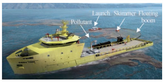Figure  1  Example of a classic pollution control vessel. (OSRV 1050, DAMEN)

Download: Full-Size Img

These boats are limited in their intervention because of their faulty hydrocarbon recovery solution that requires the extensive deployment of equipment despite unfavorable weather conditions. In addition, the delays for this deployment can easily exceed 24 hours, depending on the state of the sea. Finally, their reduced storage capacity hinders the recovery of all spilled hydrocarbons.

The progress of this recovery operation begins with a launch mainly for the deployment and towing of the boom in the polluted area, regardless of the state of the sea. Deployment of a floating boom with a maximum length of 400 m is then required to confine part of the slick such that the two ends of the boom are held one by the ship and the other by the launch to enclose the pollutant. For the recovery of hydrocarbons mixed with sea water toward the ship, a floating skimmer in the form of a volumetric screw pump fitted with a sleeve is dropped on the surface.

Owing to the slow pace of their intervention and their reduced storage capacity, hardly exceeding 1 000 m³, these classic pollution-removal vessels should be replaced by modern vessels capable of overcoming these constraints to succeed in this clean-up operation. One example is a typical vessel whose main characteristics are summarized in Table 1.

2.2   ECOCEANE concept

The company ECOCEANE specializes in the construction of small autonomous aluminum boats and collectors of solid and liquid floating waste designed for the cleaning of coastal areas, large ports, bays, and estuaries.

2.2.1   Principle underlying the ECOCEANE concept

The principle of hydrocarbon recovery is the creation of a forward flow to suck up floating pollution and a quantity of clear water through a bow door, as displayed in Figure 2.

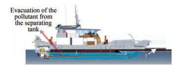Figure  2  Principle underlying the ECOCEANE concept

Download: Full-Size Img

Self-floating arms (1) are deployed to increase the collection width. In addition to the speed of the ship, a turbine is placed at the stern to facilitate the evacuation of the sea water separated from the pollutant in a separation tank (3), which is preceded by a basket (2) that filters and stops all solid waste (Figure 3).

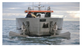Figure  3  Hydrocarbon recovery test

Download: Full-Size Img

From the tank, the flow splits into two (ECOCEANE, 2013):

1st flow: Evacuates clear water through the turbine;

2nd flow: Surface water polluted by oils and hydrocarbons passes into the separating tank, where the latter can be stored naturally without emulsion.

2.2.2   ECOCEANE pollution clean-up vessel

ECOCEANE developed its concept of recovering hydrocarbons on the high seas by offering boats of 18 m to 25 m in size, which unfortunately were not commercialized because of their low capacity. To meet market requirements, they proposed a preliminary design for a 65 m steel multimission pollution control vessel (Figure 4). Its main characteristics are summarized in Table 2.

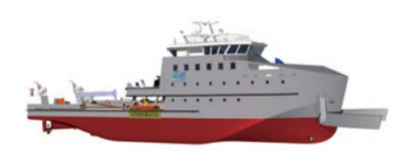Figure  4  ECOCEANE pollution control vessel

Download: Full-Size Img

However, this preliminary project was not pursued because of reliability problems. In addition, the vessel does not have the storage capacity necessary to successfully accomplish this mission. Thus, the recovery flow increase arms can be damaged in the event of bad weather. Finally, the major flaw of this concept is that it condemns a seawater tunnel from the bow door to the rear of the ship. The presence of seawater in this tunnel takes up a large amount of space on the ship and can lead to colossal maintenance and repair costs.

This concept remains effective for small tonnages and in the event of pollution in ports and estuaries. For further enhancement of the reliability of this concept, the chosen materials for the construction of this ship must be different from steel to avoid the expensive maintenance of its tunnel.

3   Innovative concept of a pollution control vessel

Historical approaches showed that conventional pollution control vessels have never succeeded in effectively controlling marine pollution problems on a global scale. Hence, their shortcomings must be reviewed and remedied to develop revolutionary, innovative, multimission pollution control vessels capable of acting quickly and efficiently to recover all the hydrocarbons spilled during a large-scale marine pollution incident, such as the case of Amoco Cadiz in 1978 (223 000 t of oil spilled) or more recently the cases of Erika in 1999 (18 000 t spilled) and Prestige in 2002 (63 000 t spilled).

3.1   Definition of the new concept

The proposed new concept offers the ECOCEANE pollution control vessel the possibility of intervening day and night by penetrating inside the oil slick without deploying equipment. Hydrocarbon recovery openings are individually equipped with a self-floating and retractable box, which acts as an arm for directing the flow inward and for containment (Figure 5).

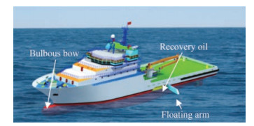Figure  5  Simulation of the launching of the new concept

Download: Full-Size Img

Taking into account all the deficiencies of the old ships, our new concept is essentially based on the results of a preliminary calculation to define its appropriate main characteristics and satisfy a storage capacity greater than 2 400 m³. The ship must be designed to accomplish other additional missions to ensure its profitability in the event of nonpollution.

For a storage capacity of more than 2 400 m³, this new concept must involve an overall ship length of 105 m without omitting the other main characteristics, which are detailed below in Table 3. To achieve this compromise and allow this ship to have certain profitability in the event of nonpollution, we are going to assign the ship with secondary missions as follows:

- Refueling at sea in the event of a crisis;

- Transport and logistics;

- Humanitarian assistance abroad;

- Medical assistance in the event of a shipwreck;

- Offshore towing; and

- Fight against the fire.

Given that the directions of the wind and current have been established beforehand, the concept allows the ship to intervene immediately upon arrival. The spacing of the arms and the speed of the vessel operating in the slick can vary between 5 and 10 kn depending on the state of the sea. Thus, the openings are individually provided with a vertical door closing upward, and the thickness of the layer at the menu surface of a heating resistor is adjusted to reduce the viscosity of the hydrocarbons and facilitate inward flow.

Hydrocarbons mixed with a small quantity of seawater are introduced without emulsion into a separator tank at two levels:

1) The lower level occupied by seawater is evacuated outside the ship using a transfer pump preceded by a separator.

2) The upper level is heated laterally by a steam coil; a skimmer floating on the surface allows the hydrocarbons to be transferred to the storage bunkers.

Accompanying waves generated by the movement of the vessel disrupt the flow of the oil recovery system and affect its efficiency. To flatten the waves around the hull and to standardize the flow upstream of the recovery openings, we equip our ship with a bulbous bow whose main objective is to reduce the resistance due to the waves of accompaniment for decreased total resistance to progress. To straighten these waves in the horizontal plane, we first choose the most appropriate bulb shape to effectively meet this objective. Second, we optimize the most suitable dimensions for the hull of the ship (Figure 6).

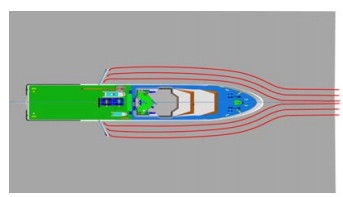Figure  6  Simulation of the intervention in the oil slick

Download: Full-Size Img

3.2   Parameters of the new pollution control vessel

When designing the ship on software, Conception Assistée Tridimensionnelle Interactive Appliquée (CATIA), we start by designing a hull that has an overall length of 82 m and fills a storage capacity of around 1 500 m³. We opt for a second design of 96 m length that offers a capacity of 2 000 m³. Ultimately, the final design of our vessel has an overall length of 105 m to achieve a storage capacity of over 2 400 m³.

We start by diagraming all the key sections that characterize the ship's hull and its bulbous bow (Figure 7) to use them in the calculations below:

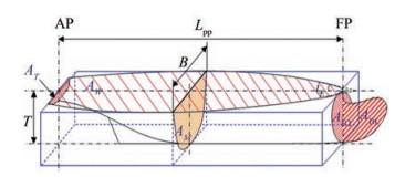Figure  7  Different sections of the hull and its bulb

Download: Full-Size Img

In the final hull design, we determine and map out the optimum and necessary key features that allow our pollution control vessel to meet the required objectives (Table 3).

4   Key bulbous bow solution for the new concept

4.1   Definition, role, and evolution of the bulbous bow

The bulbous bow is a bulge found at the front of the hull of a boat and at the level of the forefoot (junction between the bow and the keel) and constitutes an extension of the hull just below the waterline below the bow. When water flows around the hull, the bulbous bow acts as an obstacle that favors the creation of a wave out of phase with that created by the bow (Figure 8).

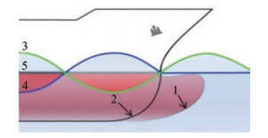Figure  8  Superposition of waves (3) and (4) in phase opposition

Download: Full-Size Img

However, the two waves coming from the bulb and the bow are in phase opposition along the hull. The superposition of these two undulations consequently cancels their effect on the hull, as displayed in Figure 8.

For the superposition to give horizontal flotation without any undulation, the phase opposition of the two waves must be perfect. For a given hull, the choice of the shape of the bulb and its dimensions must be optimized so that the two waves formed from the two obstacles are of the same amplitude and in phase opposition for a desired speed range, as displayed in Figure 9.

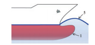Figure  9  Superposition of waves (3) and (4) cancels their effect on the hull

Download: Full-Size Img

Taylor (1943) worked on the bulbous bow by testing scale models in the US Navy's hull basin with the following fundamental hypothesis: the resistance to the progress of ships is the sum of the resistance due to the waves accompanying the ship and the viscous resistance due to friction. He quickly imagined a bulbous bow that reduces the resistance of waves at high speeds. On this initiative, the Taylor bulb quickly spread to the commercial maritime market. Since then, the competition has grown for designing and optimizing the best bulbous bow most suitable for reaching speeds of several tens of knots.

Over the years, the bulbous bow has continued to evolve from David Taylor's experiments on scale models to today's bulbous bow. Any bulge that mainly constitutes obstacles is offset from the bow to create two flows in the form of undulations in phase opposition that are superimposed in the most flattened undulation possible around the hull (Figure 10).

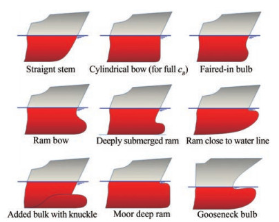Figure  10  Different shapes of bulbous bows

Download: Full-Size Img

Bulbs are classified into three types according to their cross sections, as displayed in Figure 11.

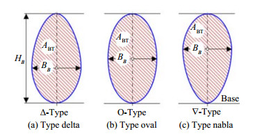Figure  11  Different types of bulbous bows according to their cross sections

Download: Full-Size Img

- Δ type: Figure 11(a) shows the drop-shaped section of the Delta type with the center of the area in the lower part. This shape can be used in large displacement longboats with low pitching motion;

- Oval type (O): This type shown in Figure 11(b) has an oval section, the center of the area in the middle, and central volumetric concentration. It is used for medium and large trips;

- ∇ type: The Nabla type shown in Figure 11(c) also has an inverted teardrop-shaped section. However, its center of the area is located in the upper half, indicating a volume concentration near the free surface. Owing to its favorable sea-keeping properties against slamming, this type is the most commonly used bulb today for small, medium, and large displacements (Weilin et al., 2017).

4.2   Significant effect of the bulbous bow on accompanying waves

When a ship moves on the surface of the water, accompanying waves form on each side at an angle of approximately 20° with the longitudinal plane of the ship (Figure 12).

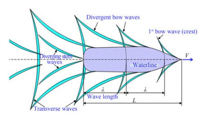Figure  12  Accompanying wave fields

Download: Full-Size Img

In this area, the two wave systems are:

- A system of transverse waves perpendicular to the axis of the ship;

- A system of divergent waves whose alignments come from the stem and the stern.

In the transverse system, the waves have the most influence on the resistance to progress (Liu et al., 2020).

On the basis of the work of Froude quoted above during a displacement of a ship, the resistance on the hull due to the accompanying waves for ships without bulbous bows increases when the undulation of the waves around the hull is evident as displayed in Figure 13. The waves that rise upfront spread entirely around the hull, requiring great power to maintain the speed of displacement. Compensating for the viscosity and mass of displaced water and the excessive consumption of fuel will enormously increase the costs.

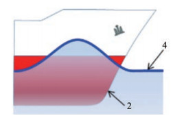Figure  13  Wave (4) generated by the bow (2)

Download: Full-Size Img

The bulbous bow also creates a wave offset from that created by the bow alone, as shown in Figure 14.

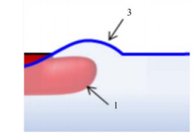Figure  14  Wave (3) generated by the bulbous bow (1)

Download: Full-Size Img

4.3   Importance of optimizing the bulbous bow in the new concept

Despite the positive bulbous bow effect, the resistance due to the accompanying waves drops but retains a significant value due to the offset of undulations (3) and (4), which are not in perfect phase opposition (Figure 15). Therefore, optimization is essential to determine the best dimensions of this bulb for the pre-established hull of our new concept so that the two waves coming out are in perfect phase opposition and the flow around the hull is perfectly horizontal for the optimal recovery of spilled hydrocarbons at high speed.

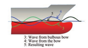Figure  15  Flow around a non-optimized bulbous bow

Download: Full-Size Img

Global research and development seek to improve and optimize the most efficient shapes to further reduce the total resistance to progress and consequently minimize consumption. The most suitable forms for this purpose are the bulb forms with Swan's Neck. This confirmation was studied and validated by Yu et al. (2010) from South Korea in an article entitled "Hull form design for the forebody of a medium-sized passenger ship with gooseneck bulb." In this work, he demonstrated that the gooseneck bow bulb is more efficient than an ordinary bulb. In the same journal, Tran (2021) from South Korea also published a study entitled "Optimal design method of bulbous bow for fishing vessels" where varying transverse and longitudinal sections of the bulb to be optimized were adopted.

5   Optimization of the bulbous bow

5.1   Objectives and constraints of optimizing the bulb design parameters

To date, no analytical approach has been established for the design of a perfect bulbous bow due to the complications of the hydrodynamic interactions between the bulb and hull. The use of numerical tools to predict hydrodynamic performance to design the perfect bulb gives the designer the opportunity to perform iterative simulations and obtain efficient results.

In accordance with the cited concept above, we apply a gooseneck bulbous bow in our depolluting boat to recover the spilled hydrocarbons at high speed. We also optimize its bulb while varying only the longitudinal sections to tailor its main dimensions specific to our pollution control vessel hull.

Since adopting a bulbous bow to improve speed and reduce drag, the designer has continued to improve its shape. This shape has evolved from the shape of a spur to the hydrodynamic shape most suited to the current situation. At this time, the most appropriate shape is the Swan's Neck shape. However, its dimensions require optimization according to the main dimensions of the assigned hull.

To meet the requirements mentioned above during the collection of hydrocarbons from the proposed pollution control vessel, we will equip this vessel with a bulbous bow in the Swan's Neck shape and optimize its longitudinal section to flatten the flow around the hull as much as possible to facilitate the recovery oil through the hull side openings (Yu et al., 2010).

The shape of the gooseneck bulb is the most appropriate shape of an obstacle that can initiate the offset of the wave created by the bow. The boss of this bulb easily generates a firm wave in its vicinity. Consequently, the two waves coming from the bulb and bow propagate along the hull in phase opposition by overlapping with a weak wave around the hull (Figure 16).

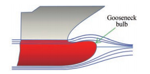Figure  16  Flow around an optimized gooseneck bulb

Download: Full-Size Img

To make the resultant of these two waves horizontal, our optimization involves adjusting the bulb L_PR length to find a horizontal flow around the hull for a speed range between 10 and 15 kn. Hence, the two waves coming from the bulb and bow are in perfect phase opposition.

In the case of our clean-up vessel with an overall length of L_OA=105 m, the bulbous bow is optimized by choosing its most modern and appropriate shape. For this purpose, the gooseneck shape with a constant Nabla (∇) cross section is chosen by varying only its L_PR length, as shown in Figure 17 (Yu, 2010; 2014; 2017).

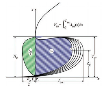Figure  17  Optimized gooseneck bulb L_PR length

Download: Full-Size Img

For the final theoretical and simulation calculation, we report the characteristics of the six best bulbs carefully chosen from an iterative simulation calculation in Table 4 below from the design of Figure 18 of the hull in 3D with the six associated bulbs while keeping the cross section constant.

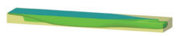Figure  18  Determination of the characteristic coefficients of the hull and its bulb

Download: Full-Size Img

The Swan's Neck shape fits the shape of the waves generated by the bulb, and the cross section in ∇ type reduces the slamming, which represents the shock with the water in the event of pitching. The justification for this choice is certainly true, but its optimization remains crucial to properly match it to the hull of our ship. Thus, this optimization is undertaken using an iterative hydrodynamic calculation and simulation to compare the results of the two methods to choose the best among the six bulbs (Rafik, 2015; Lee et al., 2005; Harun et al., 2011; Sadat-Hosseini et al., 2013; Hwuang et al., 2016; Holtrop and Mennen, 1982; Papanikolaou, 2014).

5.2   Bulb optimization using theoretical calculations

The purpose of this calculation is to choose a bulb that generates waves in phase opposition without lag relative to those generated by the hull among the six bulbs. The resultant of these two opposite waves is automatically converted to horizontal. During the intervention in the slick, the side arms in the open position will not be disturbed by the masses of water due to the accompanying waves, and the hydrocarbons flow through the side openings inwards in a laminar manner (Figure 19).

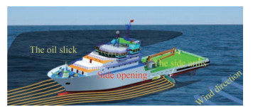Figure  19  Simulation of our pollution control vessel in action

Download: Full-Size Img

Classic hydrodynamic calculations require tests on scale models in a hull basin to deduce resistance R_W. To overcome this constraint, we use the empirical equations entitled "An approximate power prediction method" carried out by Holtrop and Mennen (1982) to calculate all the terms of the general equation of the total forward resistance (1). This method was developed using a regression analysis based on the results of experiments on 334 scale models carried out in the Netherlands Ship Model Basin. The total forward resistance R_T of the ship is subdivided into

where R_F is the frictional resistance according to Hadler (1957); 1+k₁ is form factor describing the viscous resistance of the hull form in relation to R_F; R_APP is resistance of appendages; R_W is wave-making and wave-breaking resistance; R_B is additional pressure resistance of bulbous bow near the water surface; R_TR is additional pressure resistance of immersed transom stern; and R_A is model-ship correlation resistance.

This calculation method is used for the initial bulb No.3. A numerical simulation is also carried out for the six chosen bulbs to optimize the one that generates the lowest wave resistance for a speed range between 10 and 15 kn. The results are then compared.

5.2.1   Calculation of viscous resistance

The resistance R_V = F_F(1 + k₁) remains the hydrodynamic resistance called "viscous resistance", which represents the frictional resistance (R_F) corresponding to the frictional resistance on a thin board with the same wetted surface (S_m) as the hull. Factor 1 + k₁ represents its shape coefficient.

To calculate the forces of viscosity and friction of a hull, Froude had the idea of assimilating a hull to a thin rectangular board of the same length L, wetted surface S_m, and same roughness ε. These experiments involved towing in the TORQUAY Basin thin planks of different lengths under various surface conditions to highlight a universal law of friction.

Despite his ignorance of the concept of boundary layers or the Reynolds number, he developed the method of scale models by building the first hull basin in TORQUAY that is 85 m long, 11 m wide, and 3 m deep.

Froude's ingenious idea was to separate frictional resistance from the resistance of the accompanying waves that follow the ship as it moves. The towing of thin planks of the same length and wetted surfaces as the ship does not generate waves, inspiring him first to find an empirical formula for the frictional resistance of the form (Kracht, 1978).

For the shape factor of the shell, the prediction formula is:

where C_P is prismatic coefficient of the hull from the waterline, l_cb is longitudinal position of the center of buoyancy forward of 0.5L as a percentage of L, and L_R in the form-factor formula is a parameter reflecting the length of the run according to:

The coefficient c₁₂ is defined as:

when T/L>0.05

when 0.02 < T/L < 0.05

when T/L < 0.02

where T=6 m is the mean draft and L=95 m is the length of the waterline, with T/L = 0.063 > 0.05.

For our ship:

Coefficient c₁₃ explains the specific shape of the aft shape of the ship and is related to coefficient C_stern as follows:

For coefficient C_stern, the following tentative guidelines are given in Table 5:

In our case, we adopt a U-shaped boat, so the stern shape coefficient is C_stern = 10.

The wetted area of the hull can be calculated by the empirical formula:

where C_M is the midship section coefficient, C_B the block coefficient from the waterline, C_WP the waterplane area coefficient, and A_BT is the transverse bulb area.

5.2.2   Calculation of the resistance of the appendages

The resistance of the appendages can be determined as

where ρ is the density of the water, V the speed of the ship, S_APP the total wetted surface of the appendages, 1+k₂ the resistance factor of the appendage, and C_F the friction resistance coefficient of the ship according to the Hadler (1957) and is calculated by the formula as follows:

where Re is the Reynolds number $R e=\frac{V L}{v}$, V ship's speed, ν the kinematic viscosity of seawater; and L the length of the ship's waterline.

In Table 6, provisional values of 1+k₂ are given for stream-oriented streamlined appendages. These values were obtained from strength tests with ship models with and without appendages. In several of these tests, turbulence stimulators were present at the leading edges to induce turbulent flow around the appendages.

The equivalent value 1 + k₂ for a combination of appendages is determined as:

5.2.3   Calculation of wave resistance

Finally, R_W represents the resistance of the accompanying waves that follow the ship in its movement and is determined by the formula:

where V is the ship speed, and Froude number $F n=\frac{V}{\sqrt{g L}}$,

when B/L < 0.11,

when 0.11 < B/L < 0.25,

when B/L>0.25,

For our ship:

So

where c₂ is a parameter that accounts for the reduction in wave resistance due to the action of a bulbous bow, c₅ expresses the influence of a transom stern on wave resistance, and A_T represents the submerged part of the transom area at zero speed. In this figure, the cross-sectional area of the corners placed at the transom should be included. In the wave resistance formula, Fn is the Froude number based on the waterline length L. Other parameters can be determined as follows:

when L/B < 12

when L/B>12

For our ship:

so

when C_P < 0.80

when C_P>0.80

The coefficient:

for L³/∇ < 512

Whereas

for L³/∇ > 1 727

For values of 512 < L³/∇ < 1 727, c₁₅ is determined from

and d = − 0.9.

The entry half-angle i_E is the angle measured at the waterline at the bow in degrees with respect to the vertical longitudinal plane while neglecting the local shape of the bow.

If i_E is unknown, then we can use the following formula:

Eq. (34) obtained by regression analysis of more than 200 hull shapes gives i_E values between 1° and 90°. The original equation sometimes results in negative i_E values for exceptional combinations of shell shape parameters.

The coefficient that determines the influence of the bow bulb on the resistance due to accompanying waves is defined as:

where h_B is the position of the centroid of the cross-sectional area A_BT above the keel line, and T is the ship's forward draft.

5.2.4   Calculation of resistance due to the bulbous bow

The additional resistance due to the presence of a bulbous bow near the surface is determined as

where coefficient P_B is the measurement of bulb emergence, and F_ni is the Froude number corresponding to this immersion:

and

5.2.5   Calculation of the resistance due to the transom

Similarly, the additional pressure resistance due to transom immersion can be determined as:

The coefficient c₆ is linked to the Froude number corresponding to the immersion of the transom: when Fn_T < 5

or, when F_nT≥5

Fn_T has been defined as:

where C_WP is the surface coefficient of the waterline.

5.2.6   Calculation of the model-ship correlation resistance

The model-ship correlation resistance R_A,

mainly describes the hull roughness effect and still-air resistance. From an analysis of the speed test results, which have been corrected for ideal test conditions, the following formula for the C_A correlation allocation coefficient is found:

with, when T/L ≤ 0.04

or, when T/L > 0.04

C_A could be increased to calculate the effect of hull roughness greater than a smooth hull. For this purpose, the expression from ITTC Cavitation Committee (1978) can be used, from which the increase in C_A can be derived for high values of the standard roughness of k_s=150 μm (average apparent amplitude):

6   Results of the empirical solution

Using a computer code in MATLAB, we program all the empirical formulas to calculate all these resistances. We then represent in the same graph the three predominant resistances: viscous R_V = R_F (1 + k₁), waves R_W, and total R_T. The calculation results of these different resistances for the main characteristics of the hull chosen for the initial bulb No. 3 provide data for the graph below, which represents the variation of these three resistances according to the speed of the ship as calculated in Figure 20.

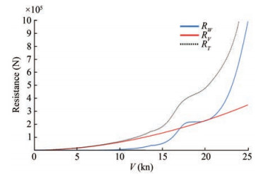Figure  20  Variation of R_W, R_V, and their resultant for the initial bulb as a function of the ship's speed

Download: Full-Size Img

According to the graph above, the variation of the viscous resistance (R_V) increases. The resistance due to the accompanying waves also increases, takes on low values between 0 and 15 kn, and becomes constant for speeds between 17 and 21 kn. Beyond 21 kn, the variation of (R_w) takes on an exponential aspect. The resultant of these two forces remains to increase at these speeds and is not completely stable similar to (R_w) for speeds between 17 and 21 kn.

In this study, the objective of this optimization is to minimize the resistance of the waves. By fixing the cross section of the bulb, we modify the longitudinal section to have six shapes of bulbs optimized beforehand. Hydrodynamic calculation is carried out to draw the curves of the resistances due to the waves of various hulls associated with the six model bulbs according to the speed.

For this purpose, the hull wave resistance R_W must be graphically simulated for the location of six associated bulbous bows. The viscous resistance remains nearly constant. Therefore, the solution to the resistance problem is to determine the minimum resistance R_W for the corresponding bulb for a displacement under full load Δ=6 400 t (Figure 21).

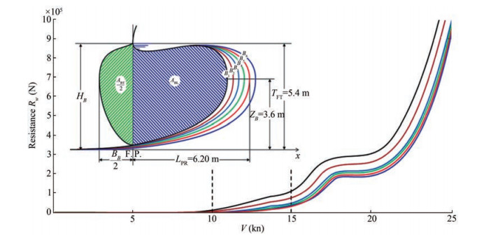Figure  21  Vessel R_W variation curves associated with different bulbs as a function of speed

Download: Full-Size Img

For the intervention speed range between 10 and 15 kn, the best results are obtained for bulbs No. 5 and No. 6. The R_W resistance of bulb No. 6 becomes optimal from a speed of 16 kn, but our major concern is more accentuated on the reduction of waves all around the ship for the speeds during the intervention than on the optimization of consumption while browsing at maximum speed. Therefore, the most desired results are those from bulb No. 5, whose dimensions are mentioned in Table 4.

6.1   Bulbous bow optimization using MAXSURF simulation

The calculation method using Holtrop's empirical equations is certainly effective. However, we do not consider the shape of the bulb associated with our vessel. Therefore, another method is used to calculate the resistance by simulation using MAXSURF software for comparison. The results obtained by simulation are almost similar to the approximate calculation.

For the optimization of the bulbous bow, this method first models the hull of the ship while assigning to it all the characteristic dimensions previously established for each of the six models of bulbs. The basic dimensions to be modified for each bulb in the form of a gooseneck are mentioned above in Table 4 for a constant cross section in Nabla (∇), as shown in Figure 22.

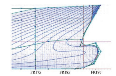Figure  22  Example of bulbous bow simulation by modifying its characteristic dimensions

Download: Full-Size Img

Once the models are formatted for the six scenarios (Figure 23), a calculation is made through successive simulations of the resistance of the corresponding accompanying waves as a function of the speed of the ship.

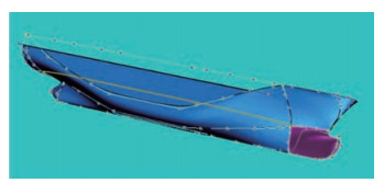Figure  23  Optimization of the most suitable bulbous bow

Download: Full-Size Img

The simulation calculation results of the resistance of the accompanying waves of the ship associated with each of the six bulbous bows are grouped in the form of curves in the same graph as shown in Figure 24. Bubbles No. 5 and No. 6 always show the best results during the simulation and thus are best suited to be associated with the hull of our ship.

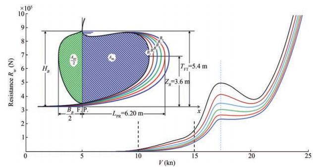Figure  24  Calculation by simulating the R_W of the ship associated with the different bulbs as a function of speed

Download: Full-Size Img

6.2   Comparison of the results of the two methods

The simulation calculation offers almost the same results as the theoretical calculation in the speed range of 10 to 15 kn. A slight difference is observed between 15 and 20 kn for the bow bulbs No. 5 and No. 6. Admittedly, bulb No. 6 offers the best results, which are close to those of bulb No. 5. Referring only to the calculation, we choose bulb No. 5 because the speed of intervention of our ship to recover the hydrocarbons is in the range between 10 and 15 kn, of which the two bulbs offer the same results.

The results obtained using the two approaches are naturally effective but are still preliminary information. For a large-scale project such as the construction of a modern multimission pollution control vessel 105 m long, tests in a hull basin remain essential to validate this optimization and definitively adjust the results obtained by simulation. Prior to any practical realization, optimization calculations are essential. This simulation work will be reinforced by a second experiment on a reduced model using the tests in hull basins associated with seven models of bulbs showing different lengths with the dimensions of bulb No. 5 taken as a reference.

7   Conclusion

Oil spills at sea are of great concern because of their negative impact on economic and ecological systems. Thus, the development of an innovative, autonomous, and multimission pollution control vessel is useful because existing antipollution vessels equipped with conventional technologies do not meet certain criteria of safety, storage capacity, and response times and are incapable of accomplishing any clean-up mission. In this study, we have described the performance of a new concept of an antipollution vessel that can meet all these requirements while performing a total and rapid recovery of spilled oil in complete safety.

The main characteristics required for this vessel have been chosen on the basis of calculations, and its gooseneck bow bulb has been optimized to have the most efficient bulb for the collection of spilled oil at high speed.

This optimization consists of adjusting the appropriate length of its bulbous bow to horizontally flatten the accompanying waves formed around the hull for reducing the total resistance to forward motion and normalizing the flow upstream of the lateral oil recovery openings. The results for the optimal bulb show that the resistance due to accompanying waves around the ship's hull is minimal for a speed range between 10 and 15 kn. Ultimately, we are confident that the obtained results demonstrate the validity of our strategy that can be adopted as soon as possible to effectively combat large-scale marine pollution.

The results obtained from this optimization are certainly effective and preliminary; however, they remain theoretical but still helpful for decision-making for small constructions. For large-scale projects such as the construction of a modern multimission antipollution ship of 105 m in length, tests in the hull basins are essential to validate and adjust the simulation results. The results of the current simulation will be verified by a second experiment on a reduced model associated with 10 bulbs of various lengths.