1   Introduction

In recent years, there is a strong demand for transforming energy supply from fossil fuels towards renewable energy sources such as solar, wind and wave. In this content, wind energy is playing a significant role as a primary source of emission-free and self-sufficient energy production. The fixed foundation wind turbine farms have been largely developed in northern Europe and in Asia (IEA, 2019). On the other hand, more than 75% of offshore wind energy resources is in waters deeper than 60 meters, where a traditional bottom-fixed offshore wind turbine is not feasible (Arent et al., 2012). To unlock the offshore potential in deeper waters for continuing efforts to decarbonise, the concepts of floating offshore wind turbine (FOWT) are seen as a promising solution (James and Ros, 2015).

Typically, the design of FOWTs is complex and requires experiments and/or simulation tools as assist verification. Compared to bottom-fixed wind turbines, the design of FOWTs is challenging, in especially the influence of platform motion on the efficiency of a FOWT under complex environmental conditions. This is because the hydrodynamic motions of a platform and the turbine motions into and out from its wake field, as well as the dynamic characterization of mooring lines, have to be considered in a coupled manner. The wave-induced motions and loads have significant influences on the efficiency of turbines and they have to be accurately predicted in design. For that reason, the hydrodynamic performance of a floating platform with mooring system then becomes the most critical aspect to be addressed firstly (Pinguet, 2021). To assess the hydrodynamics of a moored platform, mooring analysis tools have to be coupled to various hydrodynamic analysis techniques, generally classified as potential- and viscous-flow solvers (Jiang, 2021).

Although potential-flow based solvers are unable to implicitly consider viscous effects, they are widely used in marine hydrodynamics due to their robustness and computational efficiency. Typical tools based on potentialflow theory to analyze FOWTs include FAST code (Jonkman, 2007), HAWC2 (Larsen and Hansen, 2007), SIMO (Marintek, 2012) and RIFLEX (Ormberg and Passano, 2012). It is worth noting that these timedomain tools generally require the inputs of hydrodynamic coefficients from frequency-domain solvers such as WAMIT (Lee, 1995) and AQWA (ANSYS, 2016). The influence of flow viscosity can be compensated to some extend using simplified models, e. g., Morison's equations (Otter et al., 2022). Kvittem et al. (2012) studied the dynamic responses of a semisubmersible using different hydrodynamic theories. Their results showed that, in terms of motions, Morison model with forces integrated up to wave elevation gave a better prediction compared to a potential-flow model with quadratic drag forces, whose predicted motions were sensitive to the added mass coefficients.

For the floating semisubmersible type of platforms, which are being chosen for different floating offshore wind concepts, their natural frequencies of motions are generally lower than the envisaged wave-frequency band. Nevertheless, they are particularly prone to slow-drift motions. The slack catenary moorings usually result in large natural periods for surge and sway motions, which are in the range of the second-order difference-frequency excitation force (Gueydon et al., 2014). Coulling et al. (2013) found that the second-order difference-frequency wave forces were important in capturing the hydrodynamics responses of a semisubmersible. Similarly, Bayati et al. (2014) also assessed the effect of second-order hydrodynamics on a semisubmersible. They concluded that the platform's hydrodynamic responses were over predicted due to the lack of second-order difference-frequency load. Through the comparisons between various potential-flow tools and a serial benchmark OCx projects, under-predictions were at the low-frequency responses due to inaccuracies in the nonlinear difference-frequency loads (Jonkman and Musial, 2010; Robertson et al., 2014, 2016, 2020).

In general, linear and weakly nonlinear potential-flow solvers are used for the analysis of floating platforms under operational conditions, albeit with a carefully selected approach to account for viscous damping (Jiang et al., 2019, 2020). In addition, fully nonlinear potential-flow models of solving the Laplace equation have also been developed for analyzing wave-structure interactions (Grilli et al., 2001; Hague and Swan, 2009; Guerber et al., 2012; Feng and Bai, 2017). However, potential-flow methods cannot accurately predict oscillatory motions of floating structures at their natural frequencies, because viscous effects must be approximated from simplified methods (Jiang, 2021). On the other hand, these models are challenging to consider a number of key situations, where nonlinearities and complex free surface effects are prevalent (Jiang et al., 2022). In these conditions, the high-fidelity computational fluid dynamic (CFD) models have been performed to predict the motions and loads of FOWTs. Numerous CFD calculations have been performed on semisubmersibles, including decay motions in calm waters(Dunbar et al., 2015; Wang et al., 2019; Burmester et al., 2020), motions in regular waves (Pinguet et al., 2020, 2021; Rivera-Arreba et al., 2019) and focused waves (Zhou et al., 2019). Moreover, fully coupled aero-hydrodynamic analyses using CFD are also presented in the literature (Liu et al., 2017; Tran and Kim, 2015, 2016, 2018; Huang et al., 2021). It must be emphasized that the differences between these simple boundary element methods, i. e., potential-flow theory combined with Morison-type drag (referred to as BEM results in the present study) and fully nonlinear viscous-flow solvers (referred to as CFD solutions in the subsequent expressions) have been demonstrated to some extent. For instance, see Benitz et al. (2014, 2015); Tran and Kim (2015); Rivera-Arreba et al. (2019); Wang et al. (2020); Li and Bachynski-Polić (2021).

The review of research above shows that the first-order components of wave-induced motions and loads on a semisubmersible can be well predicted using BEMs. Nevertheless, due to the limit hydrodynamic modelling to linear and weakly nonlinear models, these approaches severely underpredicted the low-frequency nonlinear wave loads and dynamic responses of a semisubmersible. However, they may not capture important nonlinearities in severe sea states, which include both steep and long waves. When nonlinear phenomena are not dominant, the results obtained by BEM and CFD methods show reasonable agreement, while larger discrepancies occur for highly nonlinear regular waves. To better understand these discrepancies, a systematic comparison between results obtained from BME and CFD models is performed in the present study. Specifically, regular waves with various steepness over different frequencies are focused, which supplements the understanding in applicability of these two groups of method.

2   Numerical methods

The applied numerical methods are described in this section, consisting of the BEM code FAST v8 (Jonkman et al., 2005) and the open-source CFD library OpenFOAM v2012 (Weller et al., 1998). It stats with a brief overview of the governing equations for fluid dynamics. The rigid body dynamics is then explained. Finally, the adopted quasi-static mooring model is covered. For details of the coupling between the flow governing equations, equation of rigid body motions and mooring model, see Jiang et al. (2020); Jiang (2021); Jiang and el Moctar (2023).

2.1   Fluid dynamics

2.1.1   Potential-flow model with viscous-drag loads

A hybrid model that combines the potential-flow theory approach and the viscous-drag term from Morison's equation is adopted. Linear hydrostatic restoring, wave radiation, and diffraction forces are considered through a set of hydrodynamic coefficients based on WAMIT (Lee, 1995). The second-order potential-flow terms are included via the full set of quadratic transfer functions (QTFs). For an incompressible, inviscid, and irrotational fluid flow, its velocity potential satisfies the Laplace equation everywhere in the fluid domain:

The boundary conditions on the seabed and at the instantaneous wetted body surface S_w are given as

where n denotes distance in the direction of the unit normal vector. At the free surface, the boundary condition satisfies:

where η is the free-surface elevation. The Bernoulli equation is then derived as

where C(t) depends on the time. Choosing the ratio of the wave amplitude to wave length as the smallness parameter $\epsilon $, the perturbation approach is employed to describe the fluid potential and the fluid pressure

Consequently, the hydrostatic pressure can be determined

The first-order pressure is given as

Similarly, the second-order pressure is given as

The total forces F and moments M follow from an integration of the pressure over the instantaneous wetted surface S_w of the body (Jiang and el Moctar, 2022):

The viscous-drag loads for each member of the submerged platform geometry are calculated based on the local wave particle and structural velocities. It must be noted that only first-order wave kinematics are considered for this model, and the corresponding drag coefficients are defined based on the OC4 model description (Robertson et al., 2014).

2.1.2   Viscous-flow model

For the two incompressible and immiscible fluids, i. e. water and air in the present study, they are governed by the the continuity and the momentum conservation laws:

where v is the fluid velocity filed vector, v_m is the relative grid motion velocity vector, ν_e and ρ_e are the effective kinematic viscosity and the effective density field, and p_d is the dynamic part of pressure p:

where g is the gravity vector and r is the position vector. Then the effective density and kinematic viscosity are expressed in terms of the volume fraction α via the volume-of-fluid (VOF) method (Hirt and Nichols, 1981):

where subscripts w and a represent the water and air, respectively. The distribution and the development of the free surface is estimated using the following equation:

where v_r is a velocity field normal to the interface, standing for the artificial compression on the free surface, with its magnitude being proportional to the instantaneous velocity (Rusche, 2003). Its boundedness is insured using the Multidimensional Universal Limiter with Explicit Solution (MULES) algorithm. The forces and moments acting on the body are given as follows (Jiang and el Moctar, 2022):

where subscripts p and v denote the pressure and viscous component of the fluid-induced force and moment. p is the fluid pressure, n stands for surface normal vector of the body surface. σ^* denotes the deviatoric component of stress tensor.

2.2   Rigid body dynamics

Translations and rotations of a rigid bod are governed by the Newton-Euler equations:

where m is body mass, I is the matrix of moment of inertia in the global coordinate and ω is angular velocity.To apply the body-fixed inertia matrix $ \dot{\boldsymbol{I}}$, a transformation matrix T consisting of three consecutive Euler rotations ϕ, θ and ψ is required

The equations of motion then become as (Jiang, 2021)

where E is an identify matrix.

For potential-flow tool, the equation of motion expressed by Eq. (18) should be combined with the added mass matrix A.

Provided that the body's translation and rotation amplitudes are small, nonlinear terms of the motion equations can be neglected (el Moctar et al., 2021)

2.3   Mooring model

A quasi-static mooring model from the waves2foam tool (Jacobsen et al., 2012) is adopted in the present study to consider the catenary mooring lines. It ignores the effects of mooring dynamics, omitting the motion dependency of mass, damping and fluid acceleration on mooring lines. The mooring line shape and tension are derived from the catenary formulation. Figure 1 presents symbols describing a mooring line.

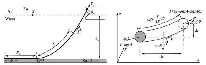Figure  1  Symbols describing a mooring line and forces acting on a differential line element, adapted from (2021)

Download: Full-Size Img

The following equations hold (Barreiro et al., 2016)

where hydrodynamic forces F and D are neglected, the mooring line is assumed to be inelastic (E=0), and the submerged weight per unit length remains constant over the entire mooring line length. The horizontal line tension at the water surface is given as:

where φ_w is the angle of the mooring lines at the water surface. And the line tension at the water surface is obtained as

It must be noted that the mooring line may have different configurations, namely the hanging state, the resting state, and the simple state. The mooring solver is implemented to restrain the moving boundary surfaces of the nonlinear rigid body motion solver, and the output values of one solver are used as input values for the other (and the opposite). An iterative approach is required to solve this coupling problem. For further details, see Barreiro et al. (2016); Jiang (2021).

3   Model description and numerical setup

3.1   Test case description

The considered test case is the OC5 semi-submersible platform (Robertson et al., 2016). The platform geometry and its coordinate system are sketched in Figure 2. A right-hand coordinate system is adopted, that is the x coordinate in forward (surge) direction; y, transverse (sway) direction; z, vertical (heave) direction. The main particulars of the floating system are summarized in Table 1, whose values are given in full scale. Note that all data and results are given at full scale in this paper, except when explicitly mentioned.

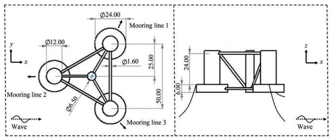Figure  2  Sketch of the OC5 DeepCwind semi-submersible platform, including its dimensions and coordinate system

Download: Full-Size Img

The experiments of the platform were performed at model scale with a scaling factor of 50, positioned using three catenary mooring lines 120° apart from each other. As shown in Figure 2, one mooring line was placed in front (line 2) and two to the sides (lines 1 and 3). Their properties are listed in Table 2.

3.2   Merical setup

The computational domain was defined by hexahedral grids, as shown in Figure 3. It consists of three layers; a uniform high-resolution middle layer extending bellow and above the still water level, encapsulating the minimum and maximum surface elevation; two layers that expand from the middle layer to the bottom and the top of the domain. The upstream and downstream domains are approximately kept as one time and four time of wave length for the simulation. The water depth was consistent with the experiments, see Table 1. The origin of the coordinate system is located at the center line of the platform and on the free surface. It must be noted that although solely the platform geometry was modelled in the present study, the whole system properties including floater, tower, nacelle, and rotor were taken into account using the full system structural properties given in Table 1. This is a common approach in simplified models of wind turbines, where the focus is on the platform's behavior rather than the detailed dynamics of the rotor and other components.

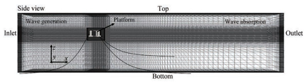Figure  3  Computational domain and the corresponding boundary conditions

Download: Full-Size Img

An overset technique was used in the present study rather than a morphing grid. This is because large motion amplitudes of the semisubmersible are expected in steep waves. According to our experiences (Jiang et al., 2020), large mesh deformations within the morphing grid technique may yield skewed shapes and unacceptable aspect ratios for grid cells, consequently inducing numerical instabilities. To overcome these limitations and still use exactly the same mesh for subsequent simulations, the overset mesh method is preferred (Jiang et al., 2021). This grid technique defines a background grid and a body-fitted grid, allowing them to move independently, and connects them at appropriate cells or points using an interpolation mechanism. Denser mesh regions are generated around the supporting platform in order to accurately capture the complex wake behaviors. The grid topology is chosen in such a way that the cell size reduces towards the floater and towards the free surface, but keeping the refinement constant in vertical direction. It worth noting that although an active wave absorption technique was used in the outlet boundary condition, a grading mesh topology was used in the extended outlet area to minimize the wave reflections.

4   Verification and validation

As the predictions from the viscous-flow solver are sensitive to temporal and spatial discretizations, the corresponding numerical errors were quantified in this section. We dispense with the verification and validation of the adopted BEM solver, as the test case was taken from a benchmark study, which has been verified and validated (Robertson et al., 2017; Wendt et al., 2019). Again, the results obtained from the BEM solver are used as comparative purpose, the high-fidelity viscous-flow solver is the main focus of current work.

4.1   Numerical errors and uncertainties

To quantify the numerical errors and uncertainties, Time-step and grid-spacing size studies were performed with a refinement factor of κ=1.5. These time-steps were defined with regard to the wave period T=2.02 s, which are $\Delta t_1=\frac{T}{900}, \Delta t_2=\frac{T}{900 \cdot \kappa}\text{ and }\Delta t_3=\frac{T}{900 \cdot \kappa^2}$. The grids were defined with regard to wave height H=0.188 m and wave length λ. Their details are listed in Table 3.

Figure 4 plots the wave elevations and the corresponding heave motions of the floater computed from three different time-step sizes with the medium grid. It should be emphasized that wave elevations were recorded at the location of the floater while excluding the floater itself. The convergence ratio R is defined as the ratio of the difference between solutions obtained on the fine (ϕ₃), and medium (ϕ₂) time-step sizes, and the difference between solutions obtained with the medium and coarse (ϕ₁) timestep sizes:

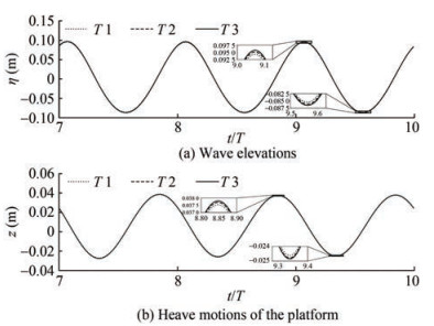Figure  4  Time-step study in terms of wave elevations and the platform heave motions computed with time-step Δt₁, Δt₂ and Δt₃ obtained on grid-spacing G₂, where η is wave elevation, z is heave motion, t is time and T is wave period

Download: Full-Size Img

For results that converged monotonically, i. e., 0 < R < 1, the Richardson extrapolation can be applied to derive the estimated numerical error δ_RE and the observed order of accuracy p_RE. With three solutions, only the leading term could be estimated, which provides the following one-term estimates:

The ratio of convergence P is applied as a measure to define the deviation of solutions from the asymptotic range:

where p_th is the theoretical order of convergence, and p_th=2 was adopted here for a second-order accuracy method. The numerical error δ_T and the numerical benchmark result ϕ_∞ are obtained as follows:

Our observed order of accuracy is limited to p_RE≥0.5 and correspondingly, a P value of close to 1 indicates grids in the asymptotic region. The uncertainty U_T was then calculated as follows (Xing and Stern, 2010):

The estimated results are listed in Table 4. We see that monotonic convergences are observed in terms of both wave elevation and heave motion. Decreasing the timestep size of Δt₂ into Δt₃ did not improve the results significantly. We chose the medium time-step of Δt₂ for our subsequent simulations.

Similarly, the comparative time histories of wave elevation and heave motion computed with grids G₁, G₂ and G₃ obtained on time-step Δt₂ are plotted in Figure 5. As seen, simulations performed on the three grids G₁, G₂ and G₃ with the selected time step Δt₂ resulted in small discrepancies, especially for heave motions obtained on the coarse grid G1. Following the same procedure, their errors and uncertainties are derived and listed in Table 5. As seen, the numerical benchmark value of ϕ_∞=0.184 5 is close to the input wave height of H=0.188 0. The similar errors ε₂ and ε₃ indicate that decreasing the grid size from medium to fine grid did not significantly improve the results. Therefore, we chose the medium grid size G₂ with time step Δt₂ for subsequent simulations.

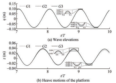Figure  5  Grid-spacing study in terms of wave elevations and the platform heave motions computed with grids G₁, G₂ and G₃ obtained on time-step Δt₂

Download: Full-Size Img

The numerical uncertainty U_SN is decomposed into error contributions from iteration number U_I, grid-spacing size U_G and time-step size U_T, which gives the following expressions for the simulation numerical error and uncertainty (Stern et al., 2017):

We dispensed with determining the iterative uncertainty, as the residual convergence criterion of 10⁻⁴ was more than satisfied. The obtained final numerical uncertainty of our simulations is U_SN=0.64%.

4.2   Comparison to experimental measurements

To validate the adopted high-fidelity numerical model and its numerical setups, hydrodynamic response were obtained from the CFD solvers are compared to experimental measurements (Robertson et al., 2016). Again, the tower and turbine were lumped into a point mass and the corre-sponding aerodynamic influence was not considered. The structure was subjected to a regular wave with a period of T=14.3 s and height of H=9.4 m.

Figure 6 plots numerically simulated and experimentally measured time histories of wave elevations and platform's motions in surge, heave and pitch. The presented time histories, respectively, consist of two parts, namely the transition states for 10 wave periods, and the stable states for two wave periods. It is worth noting that the wave elevations were nondimensionalized with respect to its theoretical wave amplitude. Their response amplitude operators (RAOs) were calculated based on these stable sections. The discrepancies between simulated and measured results are estimated and listed in Table 6. We see that, in general, good agreements were achieved in terms of wave elevations as well as the platform's motions in surge and heave. The agreement in pitch response between the CFD simulation and experimental data was not satisfactory. There could be additional factors that can influence the pitch response and contribute to the observed discrepancy between the CFD simulation and experimental data. One such factor could be the influence of experimental uncertainties, as no formal quality checks or uncertainty assessments were performed. Another possible factor may be attributed to that the whole system's moment of inertia was not correctly lumped in our simulation. And the coupled effects from the motions of other degree of freedoms during the experimental tests were more pronounced than those in our simulations. Overall, the small numerical uncertainties together with the good agreement with experimental measurements give us good confidences for our subsequent summations.

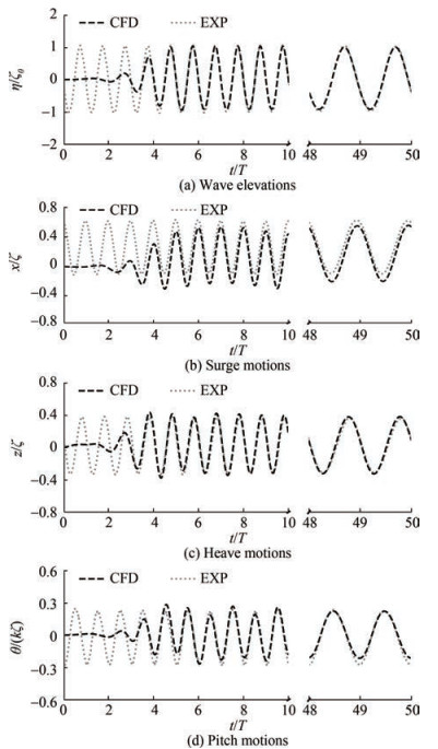Figure  6  A summary of wave elevations and platform's motions in surge, heave and pitch, where ζ is simulated wave amplitude, ζ₀ is theoretical wave amplitude, x is surge motion, θ is pitch motion and k is wave number

Download: Full-Size Img

5   Results and discussion

After the verification and validation, results obtained from the two different numerical models are systematically compared in this section. Specifically, the influences of wave steepness on wave-induced motions and loads are examined. Considered wave conditions are summarized in Table 7, where three wave frequencies of 0.518, 0.622 and 0.747 rad/s are studied. For each wave frequency, four waves with different steepness, varied from 0.032 3, 0.045 2, 0.058 8 to 0.074 5, are investigated, with steepness defined as the ratio between wave height and wave length. To show the strategy of interpreting simulation results, Figure 7 presents an exemplary time series of surge motion of the platform. Note that the motion amplitude and mean drift are analyzed separately, as mean drifts are crucial for mooring design.

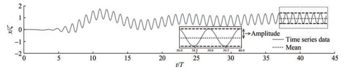Figure  7  Sample of explanatory data from the time series

Download: Full-Size Img

5.1   Motions and loads in steep waves

To demonstrate the differences between results obtained from the CFD and BEM solvers, this section presents a detailed discussion of the predicted motions and loads in a steep wave (i. e., case 8). Figure 8 plots partial time histories of computed wave elevations over five wave periods, together with their normalized amplitudes in the frequency domain. We see that a pure linear wave was generated using the BEM solver, whose wave component only exists in the wave frequency. In terms of the wave elevation computed from the CFD, due to numerical diffusion, the simulated wave height is slightly smaller than that from BEM. The nonlinear wave computed from CFD has a relatively narrow crest and a shallow but flat trough. Additionally, the second-order and third-order wave components are also observed from CFD simulations. Nevertheless, computed wave periods from both tools are idential to each other. It must be emphasised that although there are small discrepancies in the computed wave height from the two different methods, their effects on the following analysis in terms of motions and loads should be negligible, as all results are normalized using their own wave amplitudes, respectively.

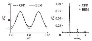Figure  8  Comparative regular wave elevations in the time and frequency domains, where ω₀ is wave frequency

Download: Full-Size Img

Figure 9 presents the associated motions in surge, heave and pitch, respectively. We see that all motions oscillate at wave frequency, and more or less the same motion responses in heave and pitch are predicted from CFD and BEM. However, in terms of responses in surge, discrepancies are observed in both amplitudes and mean drifts. The surge amplitude and mean drift obtained from BEM are both underpredicted compared to those obtained from CFD.

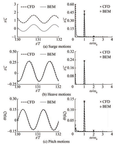Figure  9  Comparative surge, heave and pitch motion in the time and frequency domains

Download: Full-Size Img

In respect of wave-induced loads, Figure 10 plots the associated horizontal and vertical force components obtained from both solvers. It indicates that the first-order component of horizontal force predicted by the BEM solver is smaller compared to the result from the CFD solver. Nevertheless, its second-order component is larger compared to that from CFD prediction. Both of their third-order components can be negligible. Regarding the vertical forces, although discrepancies are observed in the force shapes in the time domain between BEM and CFD, barely differences are noticed in their first-order and second-order components. In general, stronger nonlinearities are detected in wave-induced loads compared to wave elevations. Highorder force components are noted, nevertheless they are much small compared to the first-order ones and their contributions to body motions are insignificant.

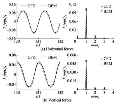Figure  10  Comparative horizontal and vertical wave force in the time and frequency domains, where F_x is horizontal wave force, F_z is vertical wave force, ρ is water density, g is gravitational acceleration and Lp is characteristic length of floater

Download: Full-Size Img

Correspondingly, Figure 11 shows the associated tensile forces acting in the fairleads of mooring line 1 (side) and line 2 (front). Note that the initial tension in calm water is excluded from these results to better demonstrate the effects of mean drift. A negative value means that the tension is smaller than the initial tension in calm water. We see that the front mooring line bears much larger forces than the side mooring lines. Compared to the results obtained from CFD, the tension amplitude and its mean value of the front line are much underpredicted by the BEM. In respect of the side line, we see that its tension amplitudes and mean value are overpredicted by the BEM. This is because the effect of mean drift was not well captured within the BEM solver. We may conclude that the design of a mooring system is dominated by a floater's surge motion, more specifically, by its low-frequency motions and mean drift.

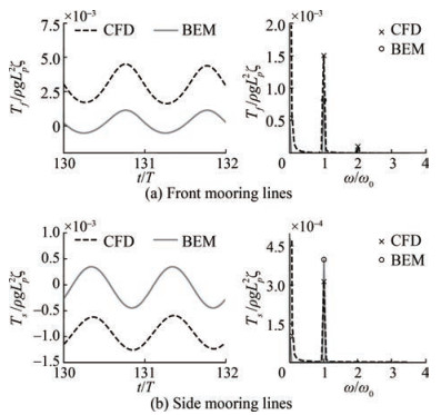Figure  11  Comparative tensile forces acting in the front and side mooring lines in the time and frequency domains, where T_f is tensile forces of front mooring, T_s is tensile forces of side mooring

Download: Full-Size Img

5.2   Effect of wave steepness

In the foregoing discussion, simulations obtained from the CFD and BEM are compared, and their discrepancies are distinguished especially in motions of mean drift and loads in mooring lines. This section gives an systematical comparison of their predictions over various wave steepness for three different wave frequencies. In terms of surge responses, Figure 12 plots the associated motion amplitudes as well as the mean drifts. We see that, for all considered wave frequencies, the wave steepness has hardly effect on surge amplitude. Favorable agreements are achieved between the CFD and BEM simulations. However, regarding the mean drifts, large discrepancies are observed for all wave frequencies, and their discrepancies become larger with the increase of wave steepness. Generally, the amplitude of surge increases but the associated mean drift decreases with the decrease of wave frequency. Specifically, the influence of wave steepness on mean drift motions is observed for BEM predictions only at ω=0.747 rad/s, while the influences are observed for all simulations from CFD. In general, the mean drift motions from BEM are very much underpredicted.

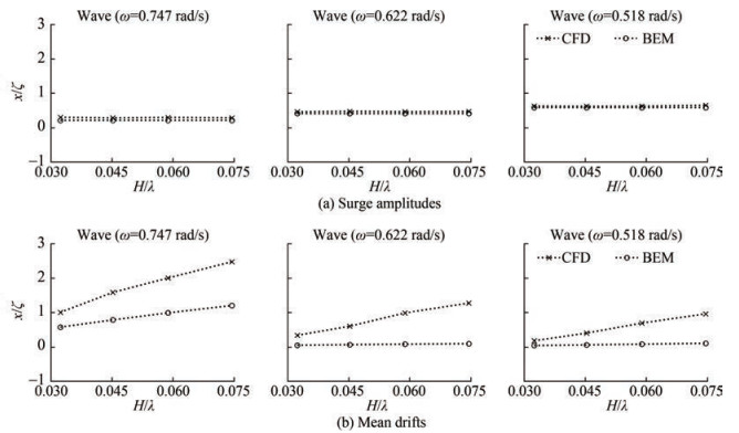Figure  12  Comparison of surge amplitudes and mean drifts over wave steepness for three different wave frequencies

Download: Full-Size Img

Figure 13 plots the influences of wave steepness on heave and pitch motions. As expected, for all considered wave frequencies, the influences of wave steepness are ignorable, although the amplitudes of heave and pitch slightly increase as the increase of wave steepness.

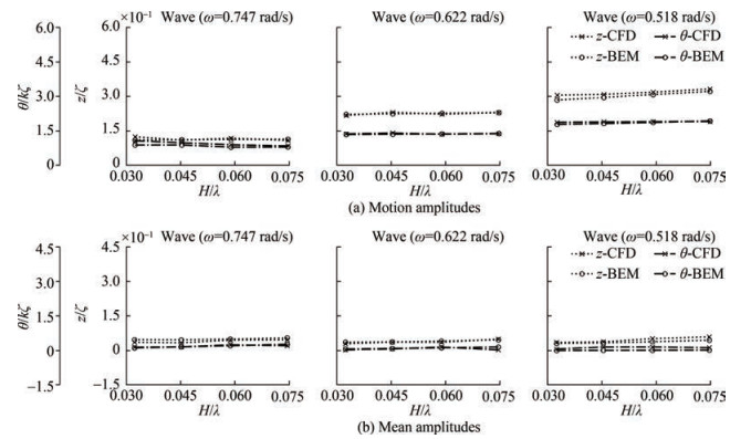Figure  13  Comparison of heave and pitch amplitudes as well as their mean values over wave steepness for three different wave frequencies

Download: Full-Size Img

Concerning the wave-induced forces in both horizontal and vertical directions shown in Figure 14, we see that the effects of wave steepness on the first-order amplitudes in both horizontal and vertical directions are insignificant. Nevertheless, effects of wave steepness are remarkable for their mean values. The mean forces in horizontal direction become larger with the increase of wave steepness. This is consist with the motions of mean drift. On the other hand, we see that the mean forces in vertical direction decrease as the wave steepness increases. Due to the existing of hydro-statics, however, their contributions to mean heave motions are minor.

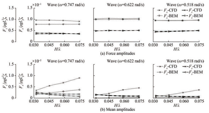Figure  14  Comparison of horizontal and vertical force amplitudes as well as their mean values over wave steepness for three different wave frequencies

Download: Full-Size Img

Finally, the tension amplitudes and their mean values of the front and side mooring lines over wave steepness are plotted in Figure 15. It indicates that the tension amplitudes of the front line increase with the increase of wave steepness. To the contrary, the tension amplitudes of the side line decrease with the increase of wave steepness. It must be noted that the effects of wave steepness on their mean values are more pronounced. Similar to their tendencies of amplitude, the mean tension acting in the front line becomes larger as the wave steepness increases. The mean tension acting in the side line decreases with the increase of wave steepness. Again, they are dominated by the motions in mean drift.

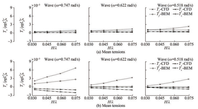Figure  15  Comparison of tension amplitudes as well as their mean values over wave steepness for three different wave frequencies

Download: Full-Size Img

6   Conclusion

We performed a comparative study of computational methods for predicting wave-induced motions and loads on a semisubmersible for various different steepness, where a fully nonlinear viscous-flow solvers and a hybrid potential-flow theory combined with Morison-type drag were used. Twelve regular waves with various steepness over three different wave frequencies are examined, with reference to the associated wave elevations and wave-induced motions and loads. In particular, the differences between the adopted two models are identified based on the predicted first-order components as well as their mean values.

Results show that when nonlinear phenomenon are not dominant, the results obtained by the hybrid model and the high-fidelity method show reasonable agreement, while larger discrepancies occur for highly nonlinear regular waves. Specifically, these discrepancies are pronounced in terms of mean drifts, resulting in a large discrepancies in their mean tensions as well. In general, the influences of wave steepness on the associated wave-induced motions and loads can be well captured using the high-fidelity viscous-flow solver. The effects of wave steepness may also be captured using the hybrid model for a certain wave frequency. Compared to the predictions obtained from the viscous-flow solver, results obtained from the hybrid model are generally smaller. We may conclude that the simplified hybrid approach may be used for the analysis under operational conditions, albeit with a carefully selected approach to account for viscous effects. Nevertheless, due to the limit hydrodynamic modelling to linear and weakly nonlinear models, these approaches severely underpredicted the lowfrequency nonlinear wave loads and dynamic responses of a semisubmersible. They may not capture important nonlinearities in severe sea states. In such conditions, a viscous-flow solver is preferred.