1   Introduction

Since the construction of the first wave tank in the Netherlands in 1956, many wave tanks have been built worldwide for the experiments of wave–body interactions. Compared with that of the open sea environment, the space of the wave tanks is limited, and the tank walls can negatively influence the experiments. For example, the reflected waves from the tank walls can travel back to the working zone and interfere with the experiments. Therefore, the waves reaching the tank walls should be absorbed to avoid reflection.

Two methods of absorbing waves are widely used in the wave tank: using a passive absorber or an active absorber. A passive absorber, such as a beach usually located at the end of the wave tank, can partially absorb incoming waves. An active absorber is a body with an external dynamic system that can perfectly absorb regular waves over a wide range of frequencies by tuning the external dynamic system. The active wave absorber was pioneered by Ursell et al. (1960). Based on the wave generation theory of Havelock (1929), they conducted an experiment and showed that 2D waves with small amplitudes can be absorbed by moving the termination at the end of the wave tank. Milgram (1970) called such devices "active water- wave absorbers" and proposed a self-actuating wave-absorbing system by determining the motion of the termination in the form of a linear operation on the measured surface elevation at a fixed point. Several different techniques have been developed for the optimal control of the active wave absorbers. They can be classified into two categories: position-control mode and force-control mode. Techniques of wave absorption can be integrated into a conventional wave maker to develop the so-called "absorbing wave maker", which can simultaneously make waves and absorb reflected waves (Hirakuchi et al., 1990).

In the position-control mode, the free surface elevations in front of the wave absorber or maker are measured to obtain incoming waves. The wave absorber or maker is moved in a manner that cancels out the incoming waves (Milgram, 1970; Christensen and Frigaard, 1994; Schäffer, 1996; Mahjouri et al., 2020). In the force-control mode, force is used as the hydrodynamic feedback mechanism. One of its advantages is that the hydrodynamic force is an integral quantity measured over the wetted body surface, thus minimizing the errors encountered with single-point measurements (Salter, 1981). Clément and Maisondieu (1993) investigated the piston wave absorber in force-control mode and first derived a frequency-dependent transfer function between the optimal velocity of the piston and the total force for the case of steady harmonic incident waves. The time-domain piston velocity leading to the complete absorption of the incident wave train was obtained by convoluting the inverse Fourier transform of the transfer function with the measured hydrodynamic force. However, the derived impulse response function of the ideal absorber is not causal and thus cannot be used as the control loop of a physical absorbing device. Therefore, they proposed two causal non-ideal approximations of this ideal noncausal controller: the Purely Unsteady Feedback-Feedforward causal approximation and the Frequency-Dependent Feedback-Feedforward causal approximation. Sub-optimal realizable controllers work remarkably well when the incident wave frequency is known. Chatry et al. (1998) proposed a self-adaptive feedback-feedforward wave absorption controller that gives good results over a broad frequency range. Other works on wave absorbers in the force-control mode were performed by Naito (2006), Spinneken and Swan (2009a, 2009b, 2009c), and Yang et al. (2015).

For the wave absorber in force-control mode, the optimal feedback force provided by the control system is dependent on the hydrodynamic forces. Therefore, the design of the wave absorber can be improved by modifying its hydrodynamic properties. For example, a reduced feedback force can lower the requirements of a mechanical system. In physical wave tanks, piston-type and flap-type wave absorbers and makers are widely used. The traditional piston-type wave absorber or maker has a draft-to-water depth ratio of 1. A feasible approach to modifying the hydrodynamic properties is to change the draft ratio. This work investigates piston-type wave absorbers with different draft ratios by focusing on the frequency-dependent hydrodynamic coefficients, the frequency-dependent transfer function between the amplitude of the optimal feedback (control) force and that of the incident regular wave, and wave absorption efficiency.

2   Governing equations and definition of wave energy absorption efficiency

The hydrodynamics of 2D piston-type active wave absorbers are investigated, and the physical model is shown in Figure 1. The depth of the wave tank is H. The piston-type active wave absorber, with a draft of l, is located at the right end of the tank. An incident wave propagating to the right (along the positive x-axis) will interact with the wave absorber and the right tank wall, resulting in the movement of the wave absorber and a wave system propagating to the left. In linear theory, the resulting wave system can be decomposed into radiation and reflected waves. The reflected wave is due to the presence of fixed obstacles. Here, the obstacles are the wave absorber and the right tank wall. The radiation wave is due to the movement of the wave absorber. The control system of the active wave absorber provides an external force (feedback or control force), modifying the motion of the wave absorber and, therefore, the radiation wave. The radiation wave should counteract the reflected wave. Ideally, the reflected wave is fully counteracted by the radiation wave, i.e., perfect absorption is achieved.

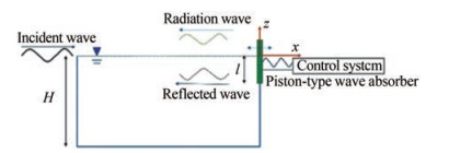Figure  1  Schematic of the physical model; the horizontal dashed line denotes the undisturbed free surface. The control system provides a feedback force that influences the motion of the water-wave absorber

Download: Full-Size Img

2.1   Governing equations for fluid flow

Assuming that the flow is irrotational and the water is incompressible and inviscid, the water flow can be represented by the potential-flow model. The velocity potential satisfying the Laplace equation, i.e., Eq. (1), is introduced. The velocity of fluid particles is given by u = ∇ϕ.

On the free surface, the kinematic and dynamic free-surface boundary conditions are satisfied: the fluid particles on the free surface always stay on the free surface, and the pressure on the free surface is equal to the atmospheric pressure. The linearized free-surface conditions are represented by Eq. (2), where η denotes the wave elevation and g the acceleration of gravity. On the wetted body surface, the impenetrable boundary condition given by Eq. (3) is satisfied; that is, the normal velocity of the fluid is equal to the normal velocity of the body. In Eq. (3), η₁ denotes the horizontal displacement of the piston, and n is the interior normal to the boundary of the water. Similarly, Eq. (4) is satisfied on the bottom or fixed tank walls.

The total velocity potential ϕ can be decomposed into the velocity potential of the incident wave ϕ_I, the velocity potential of the reflected wave ϕ_s, and the radiation velocity potential due to the motion of the wave absorber ϕ₁, i.e.,

Ideally, ϕ_s + ϕ₁ is equal to zero, i. e., the incident wave is completely absorbed. The velocity potential of a linear regular wave propagating along the positive x-axis can be expressed as

where ω, A, k and H represent the wave frequency, wave amplitude, wave number, and water depth, respectively. According to the linear wave theory, the dispersion relation, ω² = kg tanhkH, should be satisfied.

2.2   Motion of water-wave absorber

The wave force F_w, which results in the body motion, is obtained by integrating the water pressure along the wetted body surface, i. e., $ F_{w}=\int_{-1}^{0} p \mathrm{dz}$. According to Bernoulli's equation, the linearized pressure is expressed as $ p=-\rho \frac{\partial \phi}{\partial t}$. The wave force can be decomposed into the radiation force induced by the radiation wave and the diffraction force by the incident and reflected waves. In the steady state, the radiation force can be expressed as $ -A_{11}(\omega) \ddot{\eta}_{1}- B_{11}(\omega) \dot{\eta}_{1}$, where A₁₁ (ω) is the frequency-dependent added mass coefficient and B₁₁ (ω) is the wave damping coefficient. The control force, provided by the control system according to body motion, also acts on the wave absorber. For regular incident waves, the control force can be set to a damping force proportional to the body velocity plus a restoring force proportional to the body displacement, i. e., $ F_{c}=-n(\omega) \dot{\eta}_{1}-c(\omega) \eta_{1}$. Here, n(ω) and c(ω) are the damping and restoring force coefficients, respectively. Positive damping coefficients dissipate the wave energy; therefore, the incident waves are (partially) absorbed. The wave absorption efficiency can be improved by optimizing the damping and restoring the force coefficients. According to Newton's second law, the equation of motion of the wave absorber is written as

where M represents the mass of the active wave absorber, and F_D is the diffraction force (also called "wave excitation force").

2.3   Wave absorption efficiency

The wave propagating to the left consists of reflected and radiation waves. The ratio between the amplitude of the left-traveling wave and that of the incident wave, ε = A⁻ /A, is called the reflection coefficient (Milgram, 1970). When the piston is stationary, no radiation wave is present, and the piston behaves similarly to a vertical wall. Without energy loss, the amplitude of the reflected wave is equal to that of the incident wave, i. e., the total reflection. Thus, it corresponds to ε = 1. The moving piston generates a radiation wave. For positive n(ω), the radiation wave tends to offset the reflected wave, and wave absorption occurs. In such a situation, the amplitude of the left-traveling wave is smaller than that of the incident wave, resulting in ε < 1. Ideally, the incident wave is completely absorbed, corresponding to ε = 0. The average power of the control force over a wave period is $ \bar{W}=\frac{1}{T}=\int_{0}^{T} F_{c} \dot{\eta}_{1} \mathrm{~d} t=\frac{1}{2} \omega^{2} n(\omega) \eta_{1 a}^{2}$ where η_1a is the amplitude of the horizontal displacement of the piston. The power of the incident wave is the wave energy density multiplied by the group velocity of the wave expressed as $ \bar{Q}=\frac{1}{4} \rho g A^{2} \frac{\omega}{k}\left(1+\frac{2 k H}{\sinh (2 k H)}\right)$. The ratio between W and Q can represent the wave absorption efficiency.

Eq. (8) is applicable to any water depth and is the generalization of the formula given by Naito (2006) for infinite water depth. The complete wave absorption corresponds to E = 1.

3   Analytical method of piston-type wave absorber

The radiation velocity potential and the motion of the wave absorber are investigated analytically by focusing on the hydrodynamic coefficients, control force, and wave absorption efficiency.

3.1   Radiation wave

Assuming that the piston has harmonic motion in the horizontal direction, η₁ = η_1a cos ωt. The radiation velocity potential can be expressed as (Havelock, 1929)

The first term on the right-hand side of the above equation represents the left-traveling wave. The second term represents the local wave system, attenuating exponentially with increasing the distance to the piston. To satisfy the free surface condition, i. e., Eq. (2), k₀ and k_n should follow

The boundary conditions on the piston and the right tank wall can be rewritten as

Through the above equation, coefficients A₀ and A_n can be determined

Integrating the pressure $ p=-\rho \frac{\partial \phi_{1}}{\partial t}$ along the wetted surface of the piston gives the radiation force $ -A_{11}(\omega) \ddot{\eta}_{1} -B_{11}(\omega) \dot{\eta}_{1}$, which consists of an added mass force proportional to the body acceleration and a wave damping force proportional to the body velocity. The added mass and wave damping coefficients can be expressed as

Let D=l/H denote the draft (to water depth) ratio. The dimensionless added mass and wave damping coefficients at a typical water depth of 3 m with draft ratios of 1/12, 1/6, 1/3, 2/3, and 1 are presented in Figures 2 and 3. For small draft ratios, the added mass coefficient decreases rapidly with increasing frequency in the low-frequency region. Meanwhile, the wave damping coefficient increases dramatically. The smallest value of the added mass coefficients is obtained at ω = ω(l/g)^1/2 = 1.2. In the high-frequency region, the added mass coefficient varies slowly and can be approximated by the value of infinite frequency. The wave damping coefficient is extremely small.

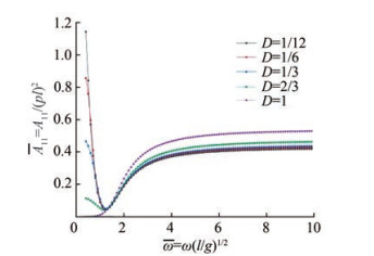Figure  2  Nondimensional added mass coefficients of piston-type wave absorber. D denotes the ratio between the draft of the piston and the water depth

Download: Full-Size Img

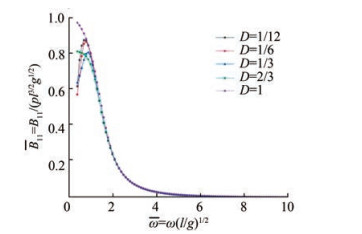Figure  3  Nondimensional wave damping coefficients of piston-type wave absorber. D denotes the ratio between the draft of the piston and the water depth

Download: Full-Size Img

3.2   Control force and wave absorption efficiency

The right wall and the piston reflect the incident wave. On the right boundary, the normal velocity induced by the incident wave is opposite to that induced by the reflected wave. Therefore, the velocity potential of the reflected wave can be written as

By integrating the pressure along the wetted surface, the diffraction force acting on the piston is expressed as

Substituting Eq. (15) into Eq. (7), we obtain the horizontal displacement of the piston η₁ = η_1a sin (ωt − β), where the amplitude and phase angle can be expressed as

and

Hence, the radiation velocity potential given by Eq. (9) becomes known. Substituting Eq. (16) into Eq. (8), we obtain

Figure 4 illustrates the wave absorption efficiency as a function of the damping coefficient n(ω) and restoring coefficient c(ω), where M = 100 kg/m, l = 0.5 m, H = 3.0 m and ω = 5.0 rad/s.

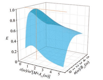Figure  4  Dependence of the wave absorption efficiency (E) on the damping coefficient n (ω) and restoring coefficient c (ω) of the control force. Here, M = 100 kg/m, l = 0.5 m, H = 3.0 m and ω = 5.0 rad/s are adopted. At the vertical orange line, a maximum wave absorption efficiency of 100% is achieved

Download: Full-Size Img

Following the approach by Bessho (1973), we obtain the maximum wave absorption efficiency at

and expresses it as

Eq. (20) indicates that perfect wave absorption can be achieved for regular incident waves. This finding corresponds to Skourup's numerical results (Skourup, 1996).

When the maximum wave absorption efficiency is achieved, the amplitude of the horizontal displacement η_1a and the phase angle β are expressed as Eq. (21). Therefore, the amplitude of the horizontal velocity is ωη_1a. Figure 5 shows the amplitudes of the horizontal displacement and velocity at the wave tank with a typical water depth of 3 m. The wave frequencies correspond to the wavelengths from 0.5 m to 6 m. With a decreasing draft ratio, the displacement and velocity amplitudes increase.

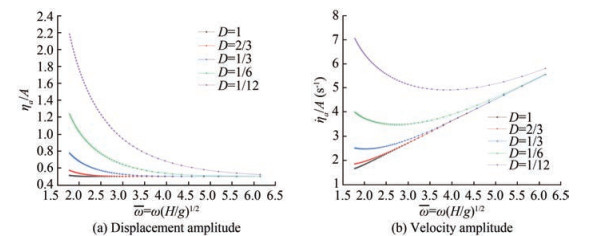Figure  5  Displacement and velocity amplitudes of pistons for the maximum wave absorption efficiency at the wave tank with a water depth of H = 3 m. η_1a is the amplitude of the horizontal velocity, A is the wave amplitude, ω the wave frequency, and D is the draft ratio of the pistons

Download: Full-Size Img

The radiation potential can be expressed as

The first term on the right-hand side of the above equation represents the left-traveling wave, which completely counteracts the left-going reflected wave. This finding is consistent with Eq. (20). The corresponding control force is

The amplitude of the control force is an interesting parameter for the design of the control system and can be represented by the transfer function given by Eq. (24).

Figure 6(a) shows the transfer function for the piston with a mass of 60 kg/m at the wave tank with a water depth of 3 m. The results for the draft ratios of D = 1/12, 1/6, 1/3, 2/3 and 1 are presented. With an increasing draft ratio, the transfer function increases significantly. For a draft ratio greater than 1/3, the required control force can be extremely large. For example, at ω = 6 (corresponding to the wavelength of 0.52 m), the required control force for the draft ratio of 1/3 is larger than 25 000 N/m2. Therefore, the required control force acting on the piston is greater than 2 500 N per unit length for an incident wave with an amplitude of 0.1 m. For the draft ratios of 2/3 and 1, the required control force at ω = 6 becomes extremely high and thus seems infeasible for application in practical wave absorbers. Figure 6(b) shows the transfer function for the draft ratios of D = 1/12, 1/6, and 1/3. The transfer function for the draft ratios of D = 1/6 and 1/12 is relatively low. The required control force acting on the piston is less than 750 N per unit length for an incident wave with an amplitude of 0.1 m in the wave frequencies of 1 ≤ ω ≤ 6 (including the interested wavelengths from 0.5 m to 6 m). This value is acceptable for the mechanical system of the wave absorbers. Reducing the draft ratio decreases the required control force but increases the amplitude of the displacement. Figure 5(a) shows that in the low-frequency region, the displacement amplitude is highly sensitive to the draft ratio and can become extremely large for a small draft ratio. The maximum displacement limits the usage of the wave absorbers with small draft ratios. Let us consider the incident wave with a wave amplitude of 0.1 m and a wavelength of 6 m (corresponding to ω = 1.77). From Figure 5(a), we found that the required displacement for D = 1/12 is about 0.22 m and that for D = 1/6 is less than 0.13 m. Assuming a maximum available displacement of 0.2 m, the draft ratio of 1/12 becomes unacceptable. For a given mechanical system of the wave absorber, small displacement amplitudes mean that waves with high amplitudes can be well absorbed. Therefore, we conclude that 1/6 can be regarded as the optimized draft ratio. Figures 6(c) and 6(d) present the results for the piston with mass M = 20 kg/m and M = 100 kg/m, respectively. The images show that the transfer function is not sensitive to the mass of the piston.

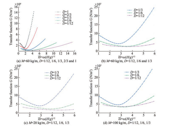Figure  6  Control-force transfer functions of the piston-type wave absorber at the wave tank with a water depth of H = 3 m. M is the mass of the piston, ω the wave frequency, and D is the draft ratio of the piston

Download: Full-Size Img

4   Numerical simulations of piston-type wave absorber

A time-domain numerical method is developed for the solutions of the hydrodynamic coefficients, control force, and wave absorption efficiency. The numerical results are compared with those obtained from theoretical analysis.

4.1   Numerical methods

The velocity potential ϕ satisfies Eq. (1), the Laplace equation. By applying Green's second identity, we can transform the Laplace equation (Eq. (1)) into the boundary integral equation (Wang et al., 2015):

where (x₀, z₀) is a field point in the fluid domain, (x, z) represents the point on the boundary, α denotes the interior angle of the boundary, and n is the normal vector positive inwards the fluid. On the free surface, ϕ is known but $ \frac{\partial \phi}{\partial n}$ is unknown. On the other boundaries, $ \frac{\partial \phi}{\partial n}$ is known through boundary conditions but ϕ is unknown. The boundary integral equation can be solved numerically by the panel method (Faltinsen, 1993).

The velocity potential ϕ can be decomposed into the incident wave ϕ_I, reflected wave, and radiation wave ϕ₁, i. e., ϕ = ϕ_I + ϕ_s + ϕ₁. The incident wave is known. In the numerical analysis, only the residual velocity potential ϕ_R = ϕ_s + ϕ₁ needs to be solved. ϕ_R involves a left-traveling wave system. When the wave system reaches the left boundary of the numerical tank, a reflected wave propagating toward the right is generated. For minimization of the right-traveling reflected wave, a damping zone is placed on the left end of the numerical tank, as shown in Figure 7.

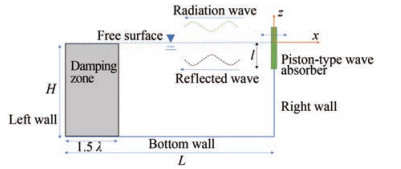Figure  7  Numerical wave tank

Download: Full-Size Img

The residual velocity potential ϕ_R is obtained by solving the boundary integral equation, which corresponds to the following boundary conditions: on the left wall and the bottom of the numerical wave tank, $ \frac{\partial \phi_{R}}{\partial n}=0$ is imposed; on the piston, $ \frac{\partial \phi_{R}}{\partial n}=-\dot{\eta}_{1}-\frac{\partial \phi_{I}}{\partial n}$ must be satisfied; on the right wall, $ \frac{\partial \phi_{R}}{\partial n}=-\frac{\partial \phi_{I}}{\partial n}$; on the free surface, ϕ_R is specified by solving the kinematic and dynamic free surface conditions represented by

In Eq. (26), γ is the artificial damping coefficient. In the damping zone,

In other regions, γ = 0. For the calculation of the hydrodynamic force, the pressure $ p=-\rho\left(\frac{\partial \phi_{R}}{\partial t}+\frac{\partial \phi_{I}}{\partial t}\right)$ is evaluated. $ \frac{\partial \phi_{R}}{\partial t}$ is unknown and needs to be solved separately. Let $ \psi=\frac{\partial \phi_{R}}{\partial t}$. This satisfies the Laplace equation

and the following boundary conditions

Integrating the pressure along the wetted surface of the piston yields $ F_{w}=-\rho \int_{-1}^{0}\left(\frac{\partial \phi_{R}}{\partial t}+\frac{\partial \phi_{I}}{\partial t}\right) \mathrm{d} z$. According to Newton's second law, the equation of motion of the piston can be expressed as

The detailed procedure for solving Eqs. (25), (26), and (33) refers to Wang and Faltinsen (2013) and Wang et al. (2015).

To obtain the added mass and wave damping coefficients of the piston, we can solve the radiation problem by neglecting the incident wave and forcing the piston to oscillate harmonically.

4.2   Numerical results

First, we solve the radiation problem by forcing η₁ = η_1a cos ωt. In the steady state, the wave force acting on the piston can be expressed as $ F_{w}(t)=-A_{11}(\omega) \ddot{\eta}_{1}- B_{11}(\omega) \dot{\eta}_{1}$. Through Fourier analysis, the added mass coefficient A₁₁ (ω) and wave damping coefficient B₁₁ (ω) at a typical water depth of 3 m are obtained. Figures 8 and 9 show the comparison of the numerical added mass and wave damping coefficients with the analytical solutions for D = 1/12 and 1. The numerical results are in good agreement with the analytical solutions.

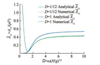Figure  8  Comparison between the numerical and analytical solutions of the added mass coefficients of the piston-type wave absorber. D = l/h denotes the draft ratio

Download: Full-Size Img

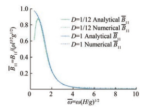Figure  9  Comparison between the numerical and analytical solutions of the wave damping coefficients of the piston-type wave absorber

Download: Full-Size Img

Once the added mass and wave damping coefficients become known, the optimized control force corresponding to the maximum wave absorption efficiency can be determined by Eq. (19). In the numerical calculation, the water depth H = 3 m, the mass of the active wave absorber M = 100 kg/m, and the dimensionless draft of the piston D = 1/6. Figure 10 shows the time history of the dimensionless wave elevations at x = − λ and x = − 2λ for the cases of A = 0.1 m and ω = 1.77 rad/s, 5.0 rad/s. The amplitude of the wave elevation corresponds to the reflection coefficient. After a few cycles, the wave elevations become negligible. This finding is consistent with the theoretical result of perfect absorption.

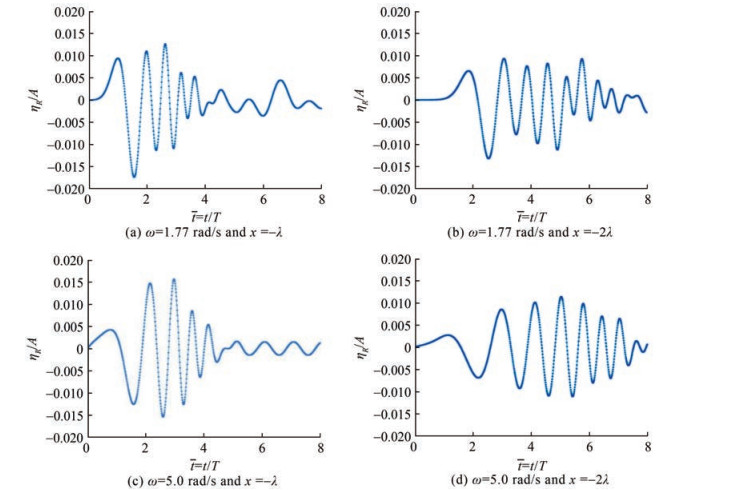Figure  10  Time history of the wave elevation. The water depth is 3 m, the amplitude of the incident wave is 0.1 m, the frequencies of the incident wave are 1.771 rad/s and 5.0 rad/s, the mass of the wave absorber is 100 kg/m, and the draft of the piston is 0.5 m

Download: Full-Size Img

Table 1 shows the wave absorption efficiency of the active wave absorber in the steady state, where the optimal damping and restoring coefficients given by Eq. (19) are adopted. The wave absorption efficiency obtained by the numerical method is close to the theoretical value of 1 (the maximum deviation is 4.3%). Figure 11 shows the transfer function between the amplitude of the optimal control force and that of the incident regular wave. The numerical solutions agree perfectly with the analytical solutions.

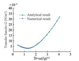Figure  11  Comparison between the analytical and numerical solutions of the transfer function of the control force. The water depth is 3 m, the mass of the wave absorber is 100 kg/m, and the draft of the piston is 0.5 m

Download: Full-Size Img

5   Conclusions

In this work, we investigated a piston-type wave absorber with different draft ratios by focusing on the frequency-dependent hydrodynamic coefficients, wave absorption efficiency, motion of the wave absorber, and control force. The analytical results were derived within the framework of the potential flow based on the linearized free-surface conditions. Results confirmed that perfect wave absorption can be achieved for regular incident waves. The draft ratio of the piston-type wave absorber strongly influences the hydrodynamic coefficients, control force, and motion of the wave absorber. The piston-type wave absorbers at the wave tank with a typical water depth of 3 m were investigated in detail, and the following results were obtained:

1) For small draft ratios, the added mass coefficient decreases rapidly with increasing frequency in the low-frequency region. Meanwhile, the wave damping coefficient increases dramatically. The smallest value of the added mass coefficients is obtained roughly at $ \bar{\omega}=\omega(l / g)^{1 / 2}=1.2$. In the high-frequency region, the added mass coefficient varies slowly and can be approximated by the value of infinite frequency. The wave damping coefficient is extremely small.

2) The dimensionless added mass $ \bar{A}_{11}=A_{11} / \rho l^{2}$ is highly sensitive to the draft ratio in the low-frequency region but becomes insensitive to the draft ratio in the high-frequency region. The wave damping coefficient is not sensitive to the draft ratio.

3) At the maximum wave absorption efficiency, the required control force can be extremely large for a draft ratio greater than 1/3. With an increasing draft ratio, the control force increases significantly. The mass of the wave absorber has a weak influence on the control force. The displacement and velocity amplitudes are sensitive to the draft ratio in the low-frequency region, increase with a decreasing draft ratio, and are independent of the mass of the wave absorber.

A time-domain numerical method based on the boundary element method was developed for the verification of the analytical solutions. Perfect agreements between the analytical solutions and the numerical results were obtained. The proposed numerical method can be used for investigating the hydrodynamic coefficients, control force, and wave absorption efficiency of active wave absorbers of any shape.