Influence of the Blocking Effect of Circulating Water Channels on Hydrodynamic Coefficient Estimation for Autonomous Underwater Vehicles
https://doi.org/10.1007/s11804-023-00354-6
-
Abstract
The Reynolds-averaged Navier–Stokes (RANS) equation was solved using computational fluid dynamics to study the effect of the circulating tank wall on the hydrodynamic coefficient of an autonomous underwater vehicle (AUV). Numerical results were compared with the experimental results in the circulating water tank of Harbin Engineering University. The numerical results of the model with different scale ratios under the same water in the flume were studied to investigate the effect of blockage on the hydrodynamic performance of AUV in the circulating flume model test. The results show that the hydrodynamic coefficient is stable with the scale reduction of the model. The influence of blocking effect on AUV is given by combining theoretical calculation with experiment.Article Highlights• In order to study the effect of blockage on the hydrodynamic performance of underwater vehicle in the model test of circulating tank, it is necessary to analyze the hydrodynamic performance by combining numerical and experimental methods.• The hydrodynamic performance of the model in the circulating tank is calculated and the hydrodynamic values under different working conditions were obtained.• The hydrodynamic performance of three models with different scale ratios is studied and the influence of blocking effect is obtained.• The results of numerical calculation are verified by experiment, which proves the accuracy of numerical calculation of hydrodynamic force. -
1 Introduction
Autonomous underwater vehicles (AUVs) play an important role in different application fields, such as marine research, environmental monitoring, and resource exploration (Wang et al., 2016; Botelho et al., 2005; Edwards et al., 2004). Establishing its precise dynamic governing equation is necessary to study the hydrodynamic performance of a submersible. However, the forces and moments in these equations are represented by hydrodynamic coefficients. Thus, numerous researchers have conducted a considerable amount of research on the method of obtaining the hydrodynamic coefficients of submersibles. Numerous methods have been reported for calculating the hydrodynamic coefficients of AUV: computational fluid dynamics (Lee et al., 2011; Qi et al., 2018; Tian et al., 2017; Randeni, 2015), experimental (Jagadeesh et al., 2009; Avila et al., 2012; Zhang et al., 2013; Chakrabarti et al., 2014; Jagadeesh et al., 2009; Krishnankutty et al., 2014; Tian et al., 2019), analytical, and semi-empirical methods (Dey et al., 2020; Kumar and Subramanian, 2007; Kepler et al., 2018; Mansoorzadeh and Javanmard, 2014), or by calculating hydrodynamic parameters to optimize performance (Wang et al., 2021; Ming et al., 2021; Yang et al., 2021). The hydrodynamic coefficients obtained by model test methods are the most accurate but are associated with many errors and uncertainties relative to other methods. For example, experimental results obtained in the towing tank are influenced by the experimental setup, the scale effect, the model, and other factors (such as manufacturing error, calibration error, and tank wall influence). By contrast, the results of numerical simulations are affected by the inaccuracy of the physical model and numerical error. Determining which method is highly accurate is difficult.
Numerous achievements have been made in predicting the hydrodynamic coefficient of AUV through model experiments or computational fluids dynamics (CFD) simulations. However, the free surface, side walls, and support bars of the towing tank or Circulating water channel (CWC) can affect the flow field and prediction accuracy; for example, the low-pressure area formed by the highspeed flow between the AUV surface and the pool wall. One study showed that reducing the model width to a tenth of the width of the pool effectively reduced the blocking effect (Kumar and Subramanian, 2007). This method ensures that the blockage effect is small but is too conservative, and a remarkably small model scale may increase the scaling effect. The effect of blockage on model resistance in a pool experiment has attracted the attention of some researchers. Kumar and Subramanian (2007) numerically simulated the influence of free surface and towing tank walls on barge resistance by using the VOF method. They maintained the size of the model constant and varied the width of the towing tank in numerical simulations. The results show that when W/B=5 (tank width W, model width B), the resistance of the selected model is unaffected by the pool wall. Liu et al. (2017) compared the results of the oblique sailing and numerical simulation tests of the KVLCC2 mode and found differences in the pressure fields around the model in the CWC and the wide flow field test.
Regarding the study of the influence of the blocking effect in the experiments, many papers have studied the influence of the pool wall on the resistance performance of the model. By referring to the towing tank experiments of others (Sun et al., 2021) in this paper, the hydrodynamic coefficients of different scale models in the same tank are obtained by the CFD method. In addition, the numerical simulation results are compared with the experimental results.
This paper is organized into five parts. Section 2 describes the test apparatus and a test model. Section 3 introduces the numerical method, and the accuracy of the numerical simulation method is verified by comparing the CFD results with experimental studies. Section 4 presents the effect of blockage on the AUV hydrodynamic coefficient. Section 5 draws the conclusion.
2 Investigation methodology
2.1 Experimental model
The shape of the AUV considered in this paper is a rectangular streamline. A fairing is installed on the front and back of the rectangular body to reduce flow separation and excessive shape resistance. The fairing was designed with practical use in mind and can be utilized as a potential ballast tank for underwater operations to store additional equipment. Figure 1 illustrates the selection process of the front and rear fairings for a streamlined model design. The bow fairing is shaped similarly to the leading edge of the NACA 0030 airfoil section. The tail fairing is a part of the NACA 0030 airfoil, which is tangential to the bottom and top of the model. The half angle α is defined as the angle at which the wing deviates from the main symmetrical horizontal plane, that is, the sweep angle of the wing. The half angle also defines the length of the tail fairing. The taper β is defined by a circular arc tangent to the side of the model. Notably, the increase of the model surface area will raise the frictional resistance, resulting in a large total resistance. Therefore, design constraints should be properly considered before modeling, which minimizes the length of the fairing while achieving low wake separation. The design featuring α = 10° and β = 30% was chosen for this project. The final design of the main body is shown in Figure 2. The length of the model is 2.23 m, the length of the bow guide cover is 0.4 m, the length of the stern guide cover is 0.63 m, the height of the model is 0.42 m and the width of the model is 0.6 m. The airfoil of the rudder is NACA0012.
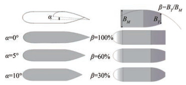 Figure 1 Model design process
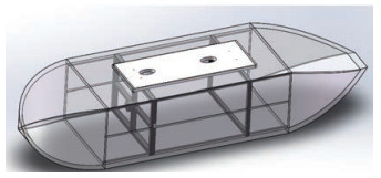 Figure 2 3D diagram of the experimental model
Figure 3 shows the model used for the model test. The model for experimental testing comprised bakelite. The structure is wrapped in fiberglass and painted with yellow paint to maintain a smooth surface and ensure the durability of the structure. The bottom of the model is cut with water holes to test the possible immersion of the model in water. The upper part of the model must be opened and drilled, and the range of activity of the balance support rod during the test is considered when opening the hole to install a fixed six-component force balance. The balance is fixed on the flange plate of the internal support plate of the model during the test.
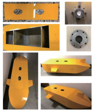 Figure 3 Model for tank test
2.2 Test device
The model test was conducted in a circulating water tank of 1.7 m×1.5 m×7 m at Harbin Engineering University. The common flow rate of the water tank is 0.3–1.6 m/s, and the maximum flow rate is 2.0 m/s. The uniform flow rate can be achieved in the cross-section of the tank, and the value of the flow rate will be displayed on the control room platform. The water tank is equipped with a honeycomb device, a rectifier network, a bubble elimination device, and a wave elimination device. When the flow rate is less than 1.5 m/s, the standing wave height is not larger than 7 mm. The standing wave refers to the failure of the experimental equipment of the pool itself to produce large standing waves under the experimental conditions of the pool in this paper, which will not affect the accuracy of the experimental results. In addition, the circulating water tank is provided with a vertical small-amplitude planar motion mechanism (as shown in Figure 4), which can provide an amplitude of 40 mm, an oscillation period of 1–5 s, an oscillation frequency of 0.2–1 Hz, and a twobar span of 400 mm. The AUV model is installed onto the VPMM through the support rod. The center of gravity of the AUV model is 0.75 m below the free water surface (as shown in Figure 5).
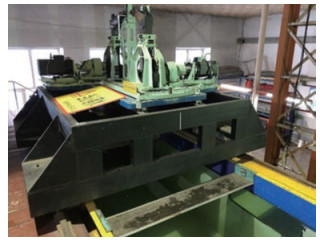 Figure 4 VPMM
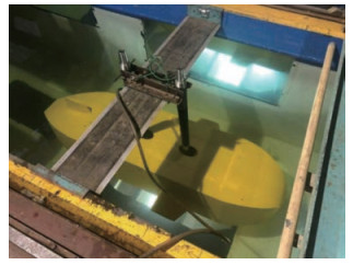 Figure 5 Model in CWC
The experiments comprise drag and static drift tests. In the drag test, the full-scale AUV is mounted under the VPMM, and the flow velocity increases from 0.3 m/s to 0.5 m/s. The data acquisition instrument will collect forces and moments in the three axial directions.
In the static drift test, the sway velocity is generated by adjusting the AUV heading angle from −10° to 10° while the flow velocity is 0.3 m/s. The forces and moments recorded on the AUV are as follows (Renilson, 2018).
$$ X=\frac{1}{2} \rho V^2 L^2 C_X $$ (1) $$ Y=\frac{1}{2} \rho L^2\left(Y^{\prime}{ }_0 u^2+Y^{\prime}{ }_v v u+Y_{v|v|}^{\prime} v|v|\right) $$ (2) $$ Z=\frac{1}{2} \rho L^2\left(Z^{\prime}{ }_0 u^2+Z^{\prime}{ }_w w u+Z^{\prime}{ }_{w|w|}{ } w|w|\right) $$ (3) $$ N=\frac{1}{2} \rho L^3\left(N^{\prime}{ }_0 u^2+N^{\prime}{ }_v v u+N^{\prime}{ }_{v|v|} v|v|\right) $$ (4) $$ M=\frac{1}{2} \rho L^3\left(M^{\prime}{ }_0 u^2+M^{\prime}{ }_w w u+M^{\prime}{ }_{w|w|} w|w|\right) $$ (5) where X, Y, and Z are forces in the x-, y-, and z-axes, respectively; L is the characteristic length, and the characteristic length of this model is selected as the total length of the model, L = 2.23 m; u, v, and w are velocities in the x, y, and z directions, respectively, because the AUV is symmetric from top to bottom, left to right; $Y^{\prime}{ }_0, Z^{\prime}{ }_0, N^{\prime}{ }_0, \text { and } M^{\prime}{ }_0$ are sufficiently small and can be ignored. L is the length of AUV, ρ is the density of fluid; $Y^{\prime}{ }_v, Y^{\prime}{ }_{v|v|}, Z^{\prime}{ }_w, Z^{\prime}{ }_{w|w|}, N^{\prime}{ }_v, N^{\prime}{ }_{v|v|}, M^{\prime}{ }_w \text {, and } M^{\prime}{ }_{w \mid w} $ are non-dimensional coefficients.
The supporting column of the pool is a long cylinder with a length of 1m and a diameter of 8 cm.
3 Numerical calculation of hydrodynamic performance
The CFD software STAR-CCM+12.02 is used to discretize the Reynolds-averaged Naivier–Stokes (RANS) equations with the second-order precision finite volume, and RANS based on the k-ε turbulence model has been solved. Turbulence model k-ε has numerous advantages, such as a fast convergence rate, low memory requirement, and good solving effect of external flow problems around complex geometry, and has been widely used in engineering practice.
3.1 Governing equation
When the fluid flow around the RANS analytical model is assumed to be incompressible, the flow equation is as follows:
$$ \operatorname{div}(\rho \boldsymbol{U})=0 $$ (6) $$ \frac{\partial\left(\rho \overline{u_i}\right)}{\partial x_i}+\frac{\partial\left(\rho \overline{u_i}~ \overline{{u}_j}\right)}{\partial x_j}=\rho \overline{f}_i-\frac{\partial \overline{p}}{\partial x_i}+\rho v \frac{\partial^2 \overline{u_i}}{\partial x_i \partial x_j}-\frac{\partial\left(\rho \overline{u_i^{\prime} u_j^{\prime}}\right)}{\partial x_i} $$ (7) where ρ is the density of the fluid, t represents time, U is the velocity vector, and u, v, and w are the magnitudes of the velocity component of U in the three axes in the three-dimensional Cartesian coordinate system. $ \overline{u_i}$ is time-mean velocity component, $ u_i^{\prime}$ is the turbulent pulsating velocity component relative to the time-mean fluid velocity, $ \bar{p}$ means pressure, $ \bar{f}_i$ is mass force component, and $ \overline{u_i^{\prime} u_j^{\prime}}$ is the mean Reynolds stress. k-ε is one of the turbulence models used to calculate Reynolds stress. The transfer equations of turbulent kinetic energy k and turbulent dissipation rate ε must be solved in this application to determine turbulent vorticity viscosity, and turbulent kinetic energy k and turbulent dissipation rate ε are defined as:
$$ \begin{aligned} & k=\frac{\overline{u_i{ }^{\prime} u_j{ }^{\prime}}}{2}=\frac{1}{2}\left(\overline{u^{\prime}}+\overline{v^{\prime 2}}+\overline{w^{\prime 2}}\right) \\ & \varepsilon=\frac{u}{\rho\left(\frac{\partial u_j^{\prime}}{\partial x_k}\right)\left(\frac{\partial u_i^{\prime}}{\partial x_k}\right)} \end{aligned} $$ (8) The transport equation of the standard k-ε model is as follows:
$$ \left\{\begin{array}{l} \frac{\partial(\rho k)}{\partial t}+\frac{\partial\left(\rho k u_i\right)}{\partial x_i}=\frac{\partial}{\partial x_j}\left[\left(\mu+\frac{\mu_t}{\sigma_k}\right) \frac{\partial k}{\partial x_j}\right] \\ +G_k+G_b-\rho \varepsilon-Y_M+S_k \\ \frac{\partial(\rho \varepsilon)}{\partial t}+\frac{\partial\left(\rho \varepsilon u_i\right)}{\partial x_i}=\frac{\partial}{\partial x_j}\left[\left(\mu+\frac{\mu_t}{\sigma_{\varepsilon}}\right) \frac{\partial \varepsilon}{\partial x_j}\right] \\ +C_{1 \varepsilon} \frac{\varepsilon}{k}\left(G_k+C_{3 \varepsilon} G_b\right)-C_{2 \varepsilon} \rho \frac{\varepsilon^2}{k}+S_{\varepsilon} \end{array}\right. $$ (9) where Gk is the turbulent kinetic energy generated by the average velocity gradient, Gb is the turbulent kinetic energy created by buoyancy, YM represents the influence of turbulence pulsation on the total dissipation rate, C1ε, C2ε and C3ε are empirical constants, σk and σε represent the Prandtl coefficient corresponding to turbulent kinetic energy and turbulence dissipation rate, respectively, and Sk and Sε are the custom source items.
3.2 Calculation of domain and boundary conditions
The size of the calculation domain during numerical calculation is equivalent to the stable flow field segment of the CWC, which has a size of 7 m×1.7 m×1.5 m, as shown in Figure 6, to simulate the real environment of the CWC. The distance to the center of the model for the origin (from the front of the computational domain) is 3 m. The model is placed in the center, and the distance between the center of the model and the upper and lower surfaces is 0.75 m. According to the actual scene of the test, the upstream and top of the calculation domain are set as velocity inlets, the downstream of the calculation domain is set as pressure outlets, and the two sides and bottom are set as no-slip walls. The surface of the hull and numerical pool wall grid is presented using multiple prismatic layer grids, as shown in Figure 7.
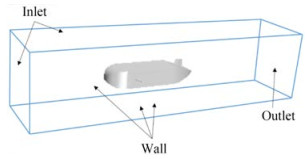 Figure 6 CWC calculation of the domain
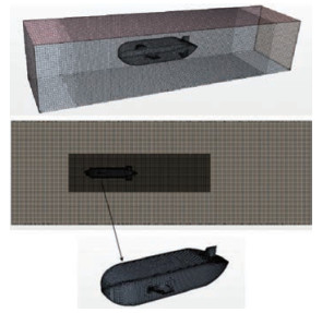 Figure 7 CWC grid diagram
The unbounded computing domain adopts the cuboid computing domain, and the volume of the rectangular domain is 6L×2L×2L (where L represents the length of the AUV vessel). The wake flow field calculation domain was 3.5L; the front of the boat is 1.5L, the hull is 1L, the pressure outlet is set 3.5L from the tail of the model, the fluid domain boundaries are set to speed entry, and the submarine is set to no-slip wall surface to simulate the AUV underwater situation. The flow field calculation domain classification is shown in Figure 8.
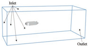 Figure 8 No blockage calculated domain
3.3 Mesh generation
The iterative solution of discrete grids will produce errors in the numerical solution. Theoretically, a fine mesh leads to a small error in the iterative results and a low sensitivity to the mesh size. However, the time cost required for the calculation will be high under a fine mesh. Choosing the appropriate mesh size during mesh division is necessary to ensure the accuracy of the calculation results and reduce the time needed for the calculation.
The cutting volume mesh is mainly used in the numerical simulation in the current study. The wall function method is utilized for the flow field at the wall surface. A dimensionless quantity y+ is introduced herein, which is defined as (Wu et al., 2014), to simulate the flow in the near wall area effectively.
$$ \begin{aligned} & y^{+}=\frac{y \sqrt{\rho \tau_w}}{\mu} \\ & {Re}=\rho U L / \mu \\ & y=L y^{+} \sqrt{80} R e^{-13 / 14} \end{aligned} $$ (10) where y is the mesh height of the first layer near the wall, τw is the wall shear force, and μ is the dynamic viscosity of a fluid. According to Equation (10), the size of y+ is related to the grid size and the fluid properties. Selection of the value of y+ should be realized on the basis of the selected turbulence model. 30 ≤ y+ ≤ 300 is generally required for the high Reynolds number model k-ε. In meshing, the thickness of the boundary layer δ should also be considered, and its calculation formula is as follows (Biringen and Chow, 2011):
$$ \delta=\frac{0.382 L}{R e^{0.2}} $$ (11) y+ = 103 based on the calculated boundary layer thickness.
The simulation calculation must set an appropriate number of grids; therefore, a grid convergence verification study is conducted. If the solution is independent of the mesh size, then the numerical results are accurate and valid. In the verification process, a group of calculation models with different numbers of grids was established, in which the height of the first layer grid was the same, to eliminate the influence on the calculation results. The number of grids in this set of computing models is 2.4×10⁵, 4.4×10⁵, 1.06 ×10⁶, 1.27×10⁶, 1.67×10⁶, and 3.31×10⁶, and the basic grids are all cut volume grids. The sailing status of the AUV is set to horizontal movement with a sailing speed of 1.2 m/s during the calculation. Figure 9 summarizes the calculation results for different mesh numbers. The convergence value is 22.056 N for 1.67 million mesh, and the resistance convergence value is 22.054 N for 3.31 million mesh. The deviation is substantially small, which indicates that further increasing the number of mesh will not affect the calculation results. This paper selects 1.67 million grids for subsequent simulation to ensure the efficiency of calculation and save the cost of calculation.
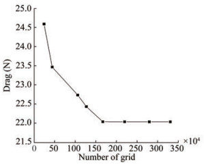 Figure 9 Grid dependency study for drag
3.4 Verification of test data
CFD modeling was performed on the CWC to compare the CFD results with the model test results and verify the accuracy of the numerical simulation. The influence of the circulating tank wall on the AUV is obtained by comparing the CWC and unbounded calculation domains.
As shown in Figure 10, the comparative data included the model experiment, CWC domain, and unbounded waters. The three aforementioned groups all predicted the AUV axial resistance at a current velocity of 0.3–1.5 m/s. Taking the solar AUV as the research object with a speed range of 0.5–1.5 m/s, the direct navigation test in the calculation domain of infinite water area and circulating water tank was numerically simulated. The statistics of the above results and model test results are shown in Table 1, and the speed is 1.5 m/s. The results of the model test, the CWC domain, and the unbounded water are 45.52, 38.72, and 33.51 N, respectively. Some differences are observed between the simulation results in the CWC domain and the model test results.
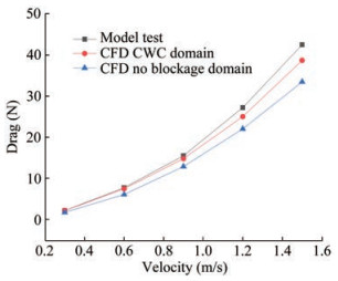 Figure 10 Comparison of CFD and drag testTable 1 Comparison of CFD and drag test (N)
Term Velocity (m/s) 0.3 0.6 0.9 1.2 1.5 Model test 2.146 7.715 15.489 27.231 42.524 CWC domain 2.139 7.456 14.781 25.039 38.723 No blockage domain 1.713 6.067 12.866 22.056 33.510 Model test results, numerical results of infinite water area, and numerical results of the calculation domain of the circulating flume were converted into dimensionless drag coefficients for comparison, as shown in Table 2, to quantify the error between the model test and numerical calculation. Error comparison revealed that the deviation of the numerical results in the calculation area of the circulating flume was 7.82%, and that of the numerical results in the infinite water area was 24.21% compared with the model test results. However, the resistance of the flume model experiment is generally larger than the result of the flume numerical simulation. This finding is due to the suspension of the real object by the experimental equipment in the real experiment and the interference of the experimental equipment in the water with the results of the model test, demonstrating a high resistance value. The resistance value of the experimental model under the no blockage domain is small due to the absence of pool wall effect under the condition of infinite water. By contrast, the numerical simulation results of the computational domain using circulating flumes are close to those of the flume experiment.
Table 2 Comparison of CFD and resistance test for the drag coefficientTerm Drag coefficient Deviation (%) Model test 0.007 347 – CWC domain 0.006 814 7.82 No blockage domain 0.005 915 24.21 In addition, a 0.45% difference exists between the results of the calculation domain prediction $Y^{\prime}{ }_v $ of circulating flume and the model test results, $N^{\prime}{ }_v $ results differ by 1.84%, $Z^{\prime}{ }_w $ results differed by 4.76%, and $M^{\prime}{ }_w $ by 6.86%. Among these results, the error mainly comes from the influence of the support column and some pool conditions. Compared with the infinite water area, the calculation results in the circulating flume area are remarkably close to the model test results. Figure 11 shows the results of the horizontal dip trial, and Figure 12 presents the results.
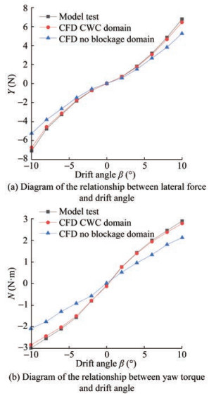 Figure 11 Comparison of CFD and resistance test for horizontal dip trial
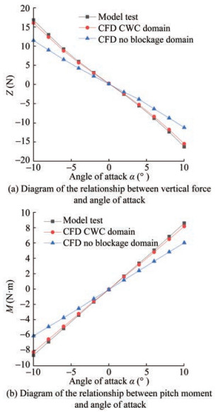 Figure 12 Comparison of CFD and resistance test for vertical dip trial
4 Numerical results and discussion
The direct course test was performed on equal-scale models with different scale ratios by the numerical simulation method to investigate the influence of the blocking effect on the direct course resistance model test in circulating flumes, and the variation law of the resistance coefficient with the model scale was also studied. The oblique sailing test was performed on the same scale models with different scale ratios using a numerical simulation method to examine the influence of the blocking effect on the corresponding hydrodynamic coefficient of the oblique sailing test. The Reynolds number and the size of the numerical circulation pool are not modified during the numerical simulation to ensure the flow similarity of the models with different scale ratios. The viscosity coefficient of the fluid in the model test in this paper is constant. Therefore, the Reynolds number can be changed by adjusting the flow rate with the experimental equipment.
4.1 Influence of the blocking effect on AUV direct flight resistance
Figure 13 shows the resistance calculation of four groups of models with different scale ratios in numerical simulation, in which the scale ratios are 1∶1, 2∶3, 1∶2, and 1∶3. In the direct flight test, the 1∶1 model was used as an example. The flow rate ranged from 0.3 m/s to 1.5 m/s, and the Reynolds number range was 6.7×10⁵ to 3.31×10⁶. The calculation results revealed that the resistance of the boat body decreases with the gradual reduction in the scale ratio. Table 3 shows the resistance coefficient obtained from the direct sailing test of models with different scale ratios, and the resistance coefficient obtained from the model with a 1∶3 scale ratio is taken as the cardinal group of the deviation term.
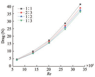 Figure 13 Drag of models with different scale ratiosTable 3 Drag coefficient of models with different scale ratios
Scale ratio Drag coefficient Deviation (%) 1∶1 0.006 814 14.24 2∶3 0.006 444 8.03 1∶2 0.006 191 3.79 1∶3 0.005 965 – 4.2 Influence of the blocking effect on AUV horizontal deviation
Table 4 describes four groups of simulations with different scale ratios, which are compared with the last group as a benchmark. The scale ratios are 1∶1, 2∶3, 1∶2, and 1∶3. The transverse force Y and the yaw moment N are shown in Figure 14. In the simulation, the Reynolds number is 6.7×10⁵, and the transverse velocity is generated by adjusting the heading angle, which varies between −10° and 10°.
Table 4 Hydrodynamic coefficient of horizontal deviationScale ratio Deviation $ Y^{\prime}{ }_v$ $ Y^{\prime}{ }_{v|v|}$ $ N^{\prime}{ }_v$ $ N^{\prime}{ }_{v|v|}$ 1∶3 Coefficient -0.072 94 -0.375 23 -0.028 97 0.024 13 1∶2 Coefficient -0.073 04 -0.403 22 -0.032 88 0.042 90 Deviation 0.14% 7.46% 13.51% 77.83% 2∶3 Coefficient -0.073 33 -0.450 95 -0.036 90 0.065 19 Deviation 0.54% 20.18% 27.39% 170.22% 1∶1 Coefficient -0.073 82 -0.532 11 -0.047 01 0.085 17 Deviation 1.20% 41.81% 62.29% 253.03% 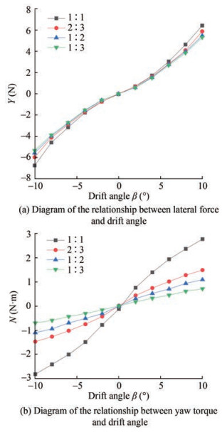 Figure 14 Results of horizontal deviation
As the scale ratio of the model decreases, $Y^{\prime}{ }_v, N^{\prime}{ }_v, Y^{\prime}{ }_{v|v|}, \text { and } N^{\prime}{ }_{v|v|} $ gradually converge to the data of the control group, and the blockage effect on second-order coefficients $Y^{\prime}{ }_{v|v|} \text { and } N^{\prime}{ }_{v|v|} $ is larger than that on first-order coefficients $ Y^{\prime}{ }_v \text { and } N^{\prime}{ }_v$. As the model size decreases, the percentage difference between $ Y^{\prime}{ }_v \text { and } N^{\prime}{ }_v$ reduces to 0.15% and 13.51%. The effect of blockage is considered in the model test, and highly accurate horizontal deviation results can be obtained by selecting an appropriate proportion.
4.3 Influence of the blocking effect on AUV vertical deviation
Table 5 describes four groups of simulations with different scale ratios, which are compared with the last group as a benchmark. The scale ratios are 1∶1, 2∶3, 1∶2, and 1∶3. Lateral force Z is shown in Figure 15, and the pitching moment N is shown in Figure 2. In the simulation, the Reynolds number is 6.7×10⁵, and the vertical velocity is generated by adjusting the pitch angle, which varies between −10° and 10°.
Table 5 Hydrodynamic coefficient of vertical deviationScale ratio Deviation $ Z^{\prime}{ }_w$ $ Z^{\prime}{ }_{w|w|}$ $ M^{\prime}{ }_w$ $ M^{\prime}{ }_{w|w|}$ 1∶3 Coefficient -0.251 99 -0.267 79 0.072 55 -0.005 40 1∶2 Coefficient -0.258 61 -0.296 53 0.074 58 -0.005 23 Deviation 2.63% 10.73% 2.80% -3.13% 2∶3 Coefficient -0.263 69 -0.377 28 0.076 80 0.004 06 Deviation 4.64% 40.89% 5.86% -175.21% 1∶1 Coefficient -0.314 69 -0.498 86 0.088 61 0.018 04 Deviation 24.88% 86.29% 22.14% -434.40% 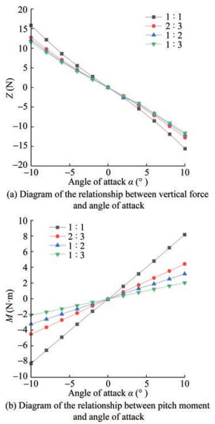 Figure 15 Results from pure sway test and pure heave tests
The reference value of the deviation in Tables 4 and 5 is the data with the model scale of 1∶3, and the calculation aims to convert the differences with the data in the first row of the table into percentages. As the scale ratio of the model decreases, $Z^{\prime}{ }_w, M^{\prime}{ }_w, Z^{\prime}{ }_{w|w|}, \text { and } M^{\prime}{ }_{w|w|} $ gradually converge to the data of the control group, and the effect of blockage on second-order coefficients $Z^{\prime}{ }_{w|w|}, \text { and } M^{\prime}{ }_{w|w|} $ is larger than that on first-order coefficients $ Z^{\prime}{ }_w, \text { and } M^{\prime}{ }_w$. As the model size decreases, the percentage difference between $ Z^{\prime}{ }_w, \text { and } M^{\prime}{ }_w$ decreases to 0.15% and 13.51%. Considering the blocking effect in the model test, a highly accurate vertical deviation result can be obtained by selecting a suitable scale model.
5 Conclusion
By comparing the data results of the circulating flume calculation domain, the infinite water area calculation domain, and the model test, the hydrodynamic coefficient obtained in the circulating flume calculation domain in this paper is close to the calculation results of the model test, in which the second-order hydrodynamic coefficient $ Y^{\prime}{ }_{v|v|}, \text { and } M^{\prime}{ }_{w|w|}$ in the oblique sailing have the largest error. When predicting the relative hydrodynamic coefficients of horizontal deviation, the errors of $Y^{\prime}{ }_v $ infinite water area are small, and those of $Y^{\prime}{ }_{v|v|}, N^{\prime}{ }_v, \text { and } N^{\prime}{ }_{v|v|} $ are large. When the correlation hydrodynamic coefficient of vertical deviation is predicted, the correlation hydrodynamic coefficient of the infinite water area is substantially large, among which the second-order hydrodynamic coefficient $M^{\prime}{ }_{w|w|} $ is the largest.
By comparing the numerical results of the models with different scale ratios under the same Reynolds number, the relevant hydrodynamic coefficients of the AUV in direct, horizontal, and vertical sailing gradually converge with the decrease in the model scaling ratio. In the horizontal sailing test, with the change in the model scale, the variation range of $Y^{\prime}{ }_v $ is the smallest and that of $N^{\prime}{ }_{v|v|} $ is the largest. In the vertical inclined navigation test, with the change in the model scale, the variation range of $Z^{\prime}{ }_w, \text { and } M^{\prime}{ }_w $ is the smallest, and that of $M^{\prime}{ }_{w|w|} $ is the largest. The smallest scale ratio of the model should be 1∶3 under the presented conditions in this paper.
Competing interest Hongde Qin is an editorial board member for the Journal of Marine Science and Application and was not involved in the editorial review, or the decision to publish this article. All authors declare that there are no other competing interests. -
Figure 1 Model design process
Figure 2 3D diagram of the experimental model
Figure 3 Model for tank test
Figure 4 VPMM
Figure 5 Model in CWC
Figure 6 CWC calculation of the domain
Figure 7 CWC grid diagram
Figure 8 No blockage calculated domain
Figure 9 Grid dependency study for drag
Figure 10 Comparison of CFD and drag test
Figure 11 Comparison of CFD and resistance test for horizontal dip trial
Figure 12 Comparison of CFD and resistance test for vertical dip trial
Figure 13 Drag of models with different scale ratios
Figure 14 Results of horizontal deviation
Figure 15 Results from pure sway test and pure heave tests
Table 1 Comparison of CFD and drag test (N)
Term Velocity (m/s) 0.3 0.6 0.9 1.2 1.5 Model test 2.146 7.715 15.489 27.231 42.524 CWC domain 2.139 7.456 14.781 25.039 38.723 No blockage domain 1.713 6.067 12.866 22.056 33.510 Table 2 Comparison of CFD and resistance test for the drag coefficient
Term Drag coefficient Deviation (%) Model test 0.007 347 – CWC domain 0.006 814 7.82 No blockage domain 0.005 915 24.21 Table 3 Drag coefficient of models with different scale ratios
Scale ratio Drag coefficient Deviation (%) 1∶1 0.006 814 14.24 2∶3 0.006 444 8.03 1∶2 0.006 191 3.79 1∶3 0.005 965 – Table 4 Hydrodynamic coefficient of horizontal deviation
Scale ratio Deviation $ Y^{\prime}{ }_v$ $ Y^{\prime}{ }_{v|v|}$ $ N^{\prime}{ }_v$ $ N^{\prime}{ }_{v|v|}$ 1∶3 Coefficient -0.072 94 -0.375 23 -0.028 97 0.024 13 1∶2 Coefficient -0.073 04 -0.403 22 -0.032 88 0.042 90 Deviation 0.14% 7.46% 13.51% 77.83% 2∶3 Coefficient -0.073 33 -0.450 95 -0.036 90 0.065 19 Deviation 0.54% 20.18% 27.39% 170.22% 1∶1 Coefficient -0.073 82 -0.532 11 -0.047 01 0.085 17 Deviation 1.20% 41.81% 62.29% 253.03% Table 5 Hydrodynamic coefficient of vertical deviation
Scale ratio Deviation $ Z^{\prime}{ }_w$ $ Z^{\prime}{ }_{w|w|}$ $ M^{\prime}{ }_w$ $ M^{\prime}{ }_{w|w|}$ 1∶3 Coefficient -0.251 99 -0.267 79 0.072 55 -0.005 40 1∶2 Coefficient -0.258 61 -0.296 53 0.074 58 -0.005 23 Deviation 2.63% 10.73% 2.80% -3.13% 2∶3 Coefficient -0.263 69 -0.377 28 0.076 80 0.004 06 Deviation 4.64% 40.89% 5.86% -175.21% 1∶1 Coefficient -0.314 69 -0.498 86 0.088 61 0.018 04 Deviation 24.88% 86.29% 22.14% -434.40% -
Avila JJ, Nishimoto K, Sampaio CM, Adamowski JC (2012) Experimental investigation of the hydrodynamic coefficients of a remotely operated vehicle using a planar motion mechanism. Journal of Offshore Mechanics & Arctic Engineering 134(2): 021601. DOI: https://doi.org/ 10.1115/1.4004952 Biringen S, Chow CY (2011) Viscous fluid flows. John Wiley & Sons, Ltd, 20–25 Botelho S, Neves R, Taddei L (2005) Localization of a fleet of AUVs using visual maps. Europe Oceans 2005 IEEE, 1320–1325 Chakrabarti R, Gelze J, Heinz L, Schmidt T (2014) Maneuverability and handling of the penguin-shaped autonomous underwater vehicle (AUV) PreToS, analytical and experimental results. OCEANS 2014, Taipei, China, 1–6 Dey S, Ali SZ, Padhi E (2020) Hydrodynamic lift on sediment particles at entrainment: Present status and its prospect. Journal of Hydraulic Engineering 145(6): 03120001. DOI: https://doi.org/ 10.1061/(ASCE)HY.1943-7900.0001751 Edwards DB, Bean TA, Odell DL, Anderson MJ (2004) A leader-follower algorithm for multiple AUV formations. 2004 IEEE/OES Autonomous Underwater Vehicles, Sebasco, 40–46. DOI: https://doi.org/10.1109/AUV.2004.1431191 Jagadeesh P, Murali K, Idichandy VG (2009) Experimental investigation of hydrodynamic force coefficients over AUV hull form. Ocean Engineering 36(1): 113–118. DOI: https://doi.org/ 10.1016/j.oceaneng.2008.11.008 Javanmard E (2013) Determination of drag and lift related coefficients of an AUV using computational and experimental fluid dynamics methods. International Journal of Maritime Engineering 62: A177–A191. DOI: https://doi.org/ 10.3940/rina.ijme.2020.a2.600 Kepler ME, Pawar S, Stilwell DJ, Brizzolara S, Neu WL (2018) Assessment of AUV hydrodynamic coefficients from analytic and semi-empirical methods. MTS/IEEE Charleston OCEANS, Charleston, 667–675 Krishnankutty P, Anantha S, Francis R, Nair PP, Krishnamachari S (2014) Experimental and numerical studies on an underwater towed body. 33rd International Conference on Ocean, Offshore and Arctic Engineering, San Francisco, V08BT06A050 Kumar M, Subramanian VA (2007) A numerical and experimental study on tank wall influences in drag estimation. Ocean Engineering 34(1): 192–205. DOI: https://doi.org/ 10.1016/j.oceaneng.2005.10.025 Liu H, Ning MA, Gu XC (2017) Calculation of the hydrodynamic forces of ship model oblique towing test in circulating water channel by considering side wall effect correction. Journal of Shanghai Jiao Tong University 51(2): 142–149. DOI: https://doi.org/ 10.16183/j.cnki.jsjtu.2017.02.003 Lee SK, Joung TH, Cheon SJ, Jang TS, Lee JH (2011) Evaluation of the added mass for a spheroid-type unmanned underwater vehicle by vertical planar motion mechanism test. International Journal of Naval Architecture & Ocean Engineering 3(3): 174–180. DOI: https://doi.org/ 10.3744/JNAOE.2011.3.3.174 Mansoorzadeh S, Javanmard E (2014) An investigation of free surface effects on drag and lift coefficients of an autonomous underwater vehicle (AUV) using computational and experimental fluid dynamics methods. Journal of Fluids & Structures 51: 161–171. DOI: https://doi.org/ 10.1016/j.jfluidstructs.2014.09.001 Qi XZ, Miao AQ, Wan DC (2018) CFD calculation of hydrodynamic derivatives of underwater vehicle. Journal of Hydrodynamics 33(3): 297–304. DOI: https://doi.org/ 10.16076/j.cnki.cjhd.2018.03.004 Randeni SAT (2015) Numerical investigation of the hydrodynamic interaction between two underwater bodies in relative motion. Applied Ocean Research 51: 14–24. DOI: https://doi.org/ 10.1016/j.apor.2015.02.006 Renilson M (2018) Submarine hydrodynamics. Springer, 130–135. https://doi.org/10.1007/978-3-319-79057-2 Sun TS, Chen GY, Yang SQ, Wang YH, Wang YZ, Tan H, Zhang LH (2021) Design and optimization of a bio-inspired hull shape for AUV by surrogate model technology. Engineering Applications of Computational Fluid Mechanics 15(1): 1057–1074. DOI: https://doi.org/ 10.1080/19942060.2021.1940287 Tian W, Mao ZY, Zhao FL, Zhao ZC (2017) Layout optimization of two autonomous underwater vehicles for drag reduction with a combined CFD and neural network method. Complexity 2017(2): 5769794. DOI: https://doi.org/ 10.1155/2017/5769794 Tian XJ, Liu YX, Liu GJ, Xie YC, Wang SQ (2019) Experimental study on influencing factors of hydrodynamic coefficient for jack-up platform. Ocean Engineering 193: 106588. DOI: https://doi.org/ 10.1016/j.oceaneng.2019.106588 Wu L, Li YP, Su SJ, Yan P, Qin Y (2014) Hydrodynamic analysis of AUV underwater docking with a cone-shaped dock under ocean currents. Ocean Engineering 85: 110–126. DOI: https://doi.org/ 10.1016/j.oceaneng.2014.04.022 Wang XY, Yang CG, Ju ZJ, Ma HB, Fu MY (2016) Robot manipulator self-identification for surrounding obstacle detection. Multimedia Tools & Applications 76(5): 6495–6520. DOI: https://doi.org/ 10.1007/s11042-016-3275-8 Wang SX, Yang M, Wang YH, Yang SQ, Lan SQ, Zhang XH (2021) Optimization of flight parameters for Petrel-L underwater glider. IEEE Journal of Oceanic Engineering 46(3): 817–828. DOI: https://doi.org/ 10.1109/JOE.2020.3030573 Yang M, Wang YH, Yang SQ, Zhang LH, Deng JJ (2021) Shape optimization of underwater glider based on approximate model technology. Applied Ocean Research 110: 102580. DOI: https://doi.org/ 10.1016/j.apor.2021.102580 Zhang XG, Zou ZJ (2013) Estimation of the hydrodynamic coefficients from captive model test results by using support vector machines. Ocean Engineering 73: 25–31. DOI: https://doi.org/ 10.1016/j.oceaneng.2013.07.007