1   Introduction

Ice is formed under extreme polar weather conditions is the major threat to the arctic marine transportation as well as polar scientific research operations. Ship-ice collision affects the normal operation of navigation (Liu et al., 2017), and even causes the ship to sink or capsize completely, seriously endangering personnel safety. The prediction of ice load is critically important in marine structure design in cold regions (Palmer et al., 2009).

However, using the simple uniaxial strength of ice to calculate ice loads is inaccurate due to the complex deformation before ice causes marine structures to fail and rupture (Zhang et al., 2019). To study the ice load on naval architectural structures (Zhang et al., 2017; Jia et al., 2019), most of the empirical design formulas or semi-empirical formulas that sum up from a large number of tension or compression experimental test (Cui et al., 2018) data are used to construct ice constitutive model equations (Snyder et al., 2016). Since they are based on many empirical assumptions, this approach has flaws in calculating the strength of ice (Mellor and Cole, 1982). Current constitutive models (Sain and Narasimhan, 2011) are difficult to provide a unified multiple scale modeling, and it is difficult to simulate the mechanical behavior of transition regions at high strain rates. Many numerical methods have been developed to predict ice failure processes (shear, melting, splitting, and fracture), showing higher efficiency than the experimental tests (Schulson, 2001). Since ice is a multiscale material with complicated physical properties, it is a challenging task to build an appropriate single scale constitutive model to facilitate accurate prediction on the ice fragmentation.

Pernas-Sanchez et al. (2015) used the Lagrangian finite element method, arbitrary Lagrangian Eulerian (ALE) method (Schulson and Buck, 1995) and Smoothed Particle Hydrodynamics (SPH) method (Sun et al., 2021; 2019; 2018) to model and simulate mechanical behavior of ice under high impacts (Kolsky, 1949), and they compared the advantages and disadvantages of the three modeling methods. Their results show that the SPH method is the most efficient method among the three methods, enabling the ice microcracks to reach a fluid-like state before creeping (Schulson and Buck, 1995; Carney et al., 2006). In addition to SPH method (Wang et al., 2006), the Discrete Element Method (DEM) also shows good performance in simulating ice loading and ice breaking properties from a macroscopic perspective, by taking into account cohesion and fragmentation effects (Gold et al., 1988; Jones, 1982; Jones, 1997). The above work, however, are within the framework of continuum mechanics, encounter great difficulties in dealing with mesoscale discontinuities, i.e. micro cracks, which are extensively occurring in the natural ice. In nature, ice is a composite material, and it is mixture of salt, air, and water (Liu et al., 2021). There are irregular bubbles (Zhang et al., 2023) in the ice interior. The existence of bubbles in the ice interior is a universal phenomenon, which affects the physical and mechanical properties of ice. Moreover, the properties of its microstructure affect its macroscopic mechanical properties (Xie and Li, 2021a; 2021b; Xie et al., 2022a; 2022b) which are also affected by temperature, salinity, porosity, and density, making it extra challenge to study. Although many efforts have been made to simulate the mechanical behavior of ice (Vazic et al., 2020), a suitable constitutive relation of ice has not been established for engineering (Han et al., 2022) applications in wide scenarios. Existing numerical methods (Li et al., 2019) simplify ice, as an isotropic uniform material, e. g. Wang et al. (2018), which ignore many key factors affecting the failure process of ice (Lu et al., 2020). More efforts are still needed to build a realistic macroscale ice constitutive model.

Recently, peridynamics method has been used to model ice destruction due to its advantages stemming from its intrinsic nonlocal formulation in dealing with discontinuities. The integral formulation of the nonlocal peridynamic theory (Silling, 2000) avoids the mathematical difficulties in evaluation of spatial derivation of the discontinuous displacement field (Madenci and Oterkus, 2014), so that it can more accurately simulate crack growth of the ice sheet in its damage state. Moreover, the state-based peridynamics can incorporate material constitutive models into mesoscale peridynamics formulation through the "force state" in the equations of motion (Silling, 2007), so that it provides a useful platform for building multiscale material constitutive models (Fan and Li, 2017a; 2017b; Fan et al., 2015; 2016).

In this work, we adopt the constitutive modeling theory of the state-based peridynamics (Hu et al., 2020), and incorporated the material constitutive model (Drucker and Prager, 1952; Johnson and Holmquist, 1994) into the integral equation form of the "force state", so as to establish a suitable and accurate mechanical model to capture ice mechanical properties over a range of multiscale. Different from the previous work, suitable ice constitutive model has been implemented into the peridynamic state equation, which can capture the multiscale mechanical responses of ice. For the microscale, peridynamics has advantages in capturing microscopic cracks in brittle materials, and it has been successfully applied in the simulation of many brittle materials such as glass (Lai et al., 2018). For the macroscale, the constitutive model used is the modified multi-surface criterion model proposed by Derradji-Aouat, the brittle failure of ice at high strain rates can be well reproduced and has many successful applications, such as ship-iceberg collisions, ship-ice interaction, and ice impact problems. The Derradji-Aouat ice constitutive model have been used to simulate the ship-iceberg collisions successfully, the proposed plastic material model yields good simulation results, both of the mesh convergence and the computational time is stable. By comparing the different inelastic constitutive models, elastic-plastic model, elastic-brittle model and the Derradji-Aouat multisurface cohesive model, the advantages and disadvantages between the three different ice constitutive models was analyzed by using the MSC.DYTRAN, and the results indicated that the multi-surface failure criterion is the most suitable one in simulation of ship-ice interaction owning to its consideration of the effects of strain rate, temperature, and hydrostatic pressure. As one of the highlights in the present peridynamic model, the influence of the added mass by water is ignored when simulating the ship-ice interaction, and the ship motion is not considered. Such issues required to be taken into account in the future work.

2   Ice constitutive model

In this section, we first briefly introduce how to incorporate ice constitutive model which is called multi-surface theory developed by Derradji-Aouat into the state-based peridynamics formulation. Then, we discuss the cohesive law used in corresponding peridynamics to determine the failure criterion for ice. Finally, a peridynamic numerical algorithm considering strain rate effect and the pressure sensitivity for simulating fresh water isotropic ice, iceberg ice and columnar saline ice is presented.

2.1   Multi-yield surface constitutive model for ice

Ice undergoes nonlinear elasto-plastic behavior at low strain rate (< 10⁻³ s⁻¹), and linear elasto-brittle failure at high strain rate (>10⁻³ s⁻¹). There is a transition zone at the strain rate (≈10⁻³ s⁻¹), the failure mode of ice is from ductile to brittle. Thus, it is an essential task to establish a suitable ice constitutive model to show the complex physical evolution during the interactions of ice with structures. To address this issue, Derradji-Aouat (2003) modified the traditional yield surface criteria by using the multi-surface theory, considerating the effects of the strain rate and the temperature of ice. It should be mentioned that this "multisurface constitutive model" has the ability to deal with not only the isotropic fresh water ice and iceberg, but also the anisotropic sea ice, which is columnar structure, as is shown in Figure 1.

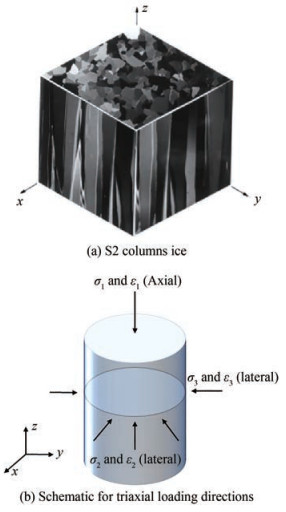Figure  1  Loading condition for columnar ice

Download: Full-Size Img

To well address this, Derradji-Aouat developed a failure criterion based on the previous data for three types of ice as is shown in Table 1, developed an elliptical yield envelop is given as the following formation:

where η, λ are the coordinates of the center point of the ellipse, P is the hydrostatic pressure, and P_max is the major axes of the ellipse, respectively. q represents the octahedral shear stress, q_max is the apex of the ellipse, Derradji-Aouat (2003) provided the q_max by the following equations:

where $ n=4, \xi=5 \times 10^{-6} \exp \left[-10.5 \times 10^3\left(\frac{1}{T}-\frac{1}{273}\right)\right]$.

In which shows the relationship between the absolute maximum octahedral shear stress q_max, the strain rate ε, and the temperature T. Eq. (2) combines the effects of strain rate and the temperature on the q_max of ice, which shows that the value of q_max increases with the increasing of the strain rate ε and the decreasing of the temperature; and decreases with the decreasing of the strain rate ε and the increasing of the temperature. In above equation,

Figure 3 shows the shape of the failure envelope proposed by Derradji-Aouat, and has been applied to model the ice materials for many years. The "Tsai-Wu" yield surface on the condition of η =0 for the isotropic material is usually written as the following form:

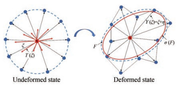Figure  2  The "state" in the non-ordinary state based peridynamics

Download: Full-Size Img

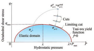Figure  3  Illustration of stress return in the Tsai-Wu yield surface (Derradji-Aouat, 2003)

Download: Full-Size Img

In which, J₂ is the second invariant for the deviatoric stress tensor, P is the Hydrostatic pressure. a₀, a₁, a₂ are constants derived from the uniaxial tensile test data. The invariant of the second-order deviatoric stress tensor can be expressed in the following form:

To describe the temperature dependent mechanical response, the corresponding change of the yield function for the ice with temperature-dependence expressed can be expressed in the following expression,

in which, T is the temperature, and linear interpolation is used to describe the temperature change from the surface of the ship and core area.

Remark 2.1  In this work, we have made several improvements over the previously-used ice constitutive model. For example, the relationship between the yield criterion and the hydrostatic pressure P is established in Eq. (5), and the relationship between the yield criterion and the material temperature T is established in Eq. (7). By doing so, the pressure sensitivity and temperature characteristics of ice are considered, which will affect the yield limit of the material.

2.2   Constitutive model in non-ordinary state based peridynamics

The multi-yield surface criterion for ice was successfully implemented in LS-DYNA software but not to its full advantage because it is difficult to deal with the discontinue problem in traditional continuum mechanics. Whereas, Peridynamics is a nonlocal mesh free method, especially for the state-based peridynamics providing a platform to integrate material constitutive model.

In the state-based peridynamics, a continuum domain Ω₀ is discretized by a set of material particle x_i with associated mass density ρ_xi and volume V_i, where i=1, 2, 3, …, ∞ is the particle index. Assume that a material particle is only influenced by forces from its neighboring particles x_j, j=1, 2, 3, …, ∞ within a local region, called as a horizon H_x(i). The horizon is typically chosen to be a circle (in 2D) or a sphere (in 3D), with the radius δ called as the horizon size of particle x_i. The relative position vector pointing from particle x_i to x_j in the reference configuration is called "bond", which can be considered as a spring in the case of elastic interaction (as shown in Figure 3), and can be denoted as:

Under certain motion or deformation χ, the continuum body deforms and the relative displacement vector in current configuration is denoted by

Then, the current relative position between these two particles can be represented by the deformation state function $ \boldsymbol{Y}\left(\xi_{i j}\right)$, which maps the undeformed bond to a deformed bond:

The peridynamic governing equation of motion, for particle x_i at time t at a reference configuration are then can be expressed as:

where ρ₀ is the mass density of the solid in the reference configuration, and $\boldsymbol{f}\left(\eta_{i j}, \xi_{i j}\right) $ is a pairwise function defined as the non-local integration of force vector that particle x_j exerts on the particle x_i as shown in Figure 3, and $\boldsymbol{b}\left(x_i, t\right) $ is the external body force density vector, as shown in Eq. (11), such particle based non-local formulation gives the peridynamics to be effective to represent discontinuity everywhere.

In the Peridynamics theory, besides the deformation state $\underline{\boldsymbol{Y}} $, another concern is the force state $\underline{\boldsymbol{T}} $, with which the balance of the momentum is expressed as:

In this work, the state-based Peridynamics theory takes strain-rate effects into account. The governing equation can be expressed as follows:

We can obtain the relation between the force-vector state T and the first Piola-Kirchhoff stress tensor P_xi of classical continuum mechanics as:

where ω(ξ_ij) is a positive scalar influence function defined on the bond length of each material bond ξ_ij, which is the distance of the two particles, and K_xi is the reference symmetric shape tensor of particle x_i which can be defined as:

If the horizon size of the particle x_i is the same as that of the particle x_j, assume that the deformations of all the bonds ξ_ij within a horizon H_xi is uniform, we have $ \boldsymbol{K}_{x_i}=\boldsymbol{K}_{x_j}$. Based on continuum mechanics, the relation between P_xi and the Cauchy stress σ_xi is written by

where F_xi is the non-local deformation gradient at the particle x_i.

In order to obtain the first Piola-Kirchhoff stress P_xi, we should first obtain the deformation gradient tensor F_xi and its time derivative $\dot{\boldsymbol{F}}_{x_i} $, the velocity tensor, $ \boldsymbol{L}=\dot{\boldsymbol{F}} \boldsymbol{F}^{-1}$, and the rate of deformation tensor $\boldsymbol{D}=\frac{1}{2}\left(\boldsymbol{L}+\boldsymbol{L}^{\mathrm{T}}\right) $. Then based the hypo-elastic-plastic formulation that will be discussed in the next Section, we can find the Cauchy stress σ.

Here, we first discuss the construction of the nonlocal deformation gradient. The deformation gradient in a material point from the initial configuration to the current configuration is described by the deformation gradient. For quasi-uniform particle distributions, the corresponding deformed bonds can be expressed as:

where F_xi is a second-order tensor and it can be viewed as the approximated deformation gradient at the particle x_i. Then we can obtain,

Then the nonlocal deformation gradient F_xi defined at the particle x_i in terms of shape tensors can be obtained as:

The spatial velocity gradient satisfies the following relationship:

in which, $ \dot{\boldsymbol{F}}$ is the time derivative of the deformation gradient, defined as:

The spatial velocity gradient L can be decomposed into a symmetric deformation rate tensor D and an asymmetric rotation tensor W:

The material frame-indifference criterion imposes the objectivity condition, and the constitutive model must be invariant within a certain range. Therefore, only objective quantities can be used in the constitutive model.

In this work, we adopt the Hughes-Winget formula (Hughes and Winget, 1980; Rubinstein and Atluri, 1983) in the stress update under large deformation condition. First, the rate of deformation tensor d is calculated as,

where R_t is an orthogonal rotation tensor, which is used to describe the rotation of the rigid body at time t, and it can be expressed by the following incremental formula:

where $ \varOmega^2=\omega_i \omega_j \text { and } \varOmega_{i j}=\mathrm{e}_{i k j} \omega_k$ is the tensor sequence number, e_ikj is the axial vector can be expressed as:

in which, the vorticity $\boldsymbol{w}=-\frac{1}{2} e_{i j k} \boldsymbol{W}_{j k} \boldsymbol{e}_i, \boldsymbol{z}=e_{i k j} D_{j m} V_{m k} \boldsymbol{e}_i $, the left stretch tensor can be expressed as:

where $ \dot{\boldsymbol{V}}_{\Delta t}=\boldsymbol{L} \dot{\boldsymbol{V}}_t-\dot{\boldsymbol{V}}_t \varOmega$ is the left stretch rate tensor at each time step, which can be used to V and R.

After the rate of deformation tensor d is being calculated, the Cauchy stress, von-Mises stress, and plastic strain can be calculated subsequently. Therefore, the Cauchy stress of the material can be obtained from the following formula:

Then we can calculate the first Piola-Kirchhoff stress tensor as follows,

where $ J=\operatorname{det} \boldsymbol{F}_{x_i}$.

Remark 2.2  In this work, we incorporated Eq. (28) into the state-based peridynamics to find the bond force states, after we find the Cauchy stress that is determined by the ice constitutive model. Thus, the ice constitutive model can be incorporated through Eq. (28) into the framework of the state-based peridynamics.

2.3   Plastic response for ice in the framework of peridynamics

According to the plastic flow law, under ideal conditions, the surface of the plastic region and the yield surface coincide. Therefore, the plastic potential function based on the Derradji-Aouat (DA) constitutive model can be expressed as follows,

where $ \|\boldsymbol{s}\|$ denotes the scalar of deviator stress tensor; a₀ a₁, a₂ are the experimental constant.

The hydrostatic pressure can be expressed as:

where I is the unit second order tensor. The deviatoric stress tensor can be obtained by the following formula,

in which, σ is the stress tensor.

In order to describe the material deformation. The deformation rate tensor is decomposed into the elastic part, the plastic part and the temperature part, respectively, and can be denoted as:

The relationship between the elastic deformation rate tensor and elastic stress in the above formula satisfies:

in which, $ \sigma^{\nabla}$ is the true objective stress rate tensor, C^e is the elasticity coefficient tensor. In order to facilitate the subsequent derivation, the elastic coefficient tensor can be expressed as:

where K is the yield modulus of the material, G is the shear modulus of the material. Generally, the value of the true equivalent stress can be obtained from the following formula:

The true plastic strain rate can be obtained from the following equation:

Substituting Eq. (35) into Eq. (31):

where n is the direction vector of deviator stress tensor, and I is the second-order unit tensor:

Therefore, according to the plastic flow law, the plastic part of the deformation rate d^p in Eq. (32) can be expressed as the product of the plastic consistency parameter term γ and the derivative of the plastic potential function $ \frac{\partial \varPhi}{\partial \sigma}$ as follows:

where $ s=\|\boldsymbol{s}\|$.

Under the condition that the material is deformed by rotation, the regression mapping format is used for processing. Figure 2 shows a schematic diagram of the regression mapping method. In the process of spatial integration, the integral increment of the constitutive model can be regarded as a kind of "strain-driven" process, and all the strain tensor increments at the orthogonal point will update the stress at time t. The Newton-Raphson algorithm is used to solve the nonlinear equations. Because a fully implicit solver consumes computational time, we used a semi-implicit integration format to solve the integral equations. In computations, at time step n+1, the envelope of inelastic flow can be estimated by the yield function and the plastic potential function, and the corresponding updated stress is given as:

In the formula, the test stress can be calculated by the following formula:

where σ_n is the stress at time step n, Δd is the total deformation increment.

The return increment of stress Δσ^re can be expressed as:

where Δγ is the plastic consistency parameter increment. Therefore, the test stress is updated to the following expression:

The stress is updated to the following expression:

In the process of the iterative solution, the deformation of the material first undergoes an elastic phase, and then plastic deformation occurs after the elastic phase. The elastic and plastic phases are judged by the yield equation. The material reaches the yield condition at the Gauss integration point. The yield equation at the n+1 time step is written as follows:

If $ f_{n+1}^{\text {trial }}<0$, the material enters the elastic phase; if $f_{n+1}^{\text {trial }} \geqslant 0 $, the material enters the plastic phase. As a result, the expression of the plastic consistency parameter increment Δγ used to solve the return value increment of the stress in Eq. (43) can be obtained:

The return increment value of the true equivalent stress can be solved by the increment of the plastic consistency parameter as:

The return increment value of the pressure is solved by the plastic consistency parameter increment, which can be expressed as follows:

From Eq. (48) to Eq. (49), the expression of the envelope$\{p, \bar{\sigma}\} $of the two-dimensional space can be obtained:

Finally, the updated equivalent plastic strain is obtained by using the plastic consistency parameter increment to solve the expression:

The hydrostatic pressure can be expressed as follows:

Therefore, the unrotated Cauchy stress including deviatoric stress and hydrostatic pressure is expressed by the formula in Eq. (28). The unrotated Cauchy stress needs to be the rotating Cauchy stress. Finally, the unrotated Cauchy stress tensor of the material can be calculated by the following equation:

Then the real Von-Mises stress at time t is updated as:

Remark 2.3  One of the main features of the proposed peridynamics model is that the updated multi-yield surface criterion shown in Eq. (50) is used to calculate inelastic stress of the ice. Ice will be under plastic deformation when $f_{n+1}^{\text {trial }} \geqslant 0 $, as is shown in Figure 3, and the plastic response can be calculated by Eq. (58).

2.4   Damage model for ice

In peridynamics, the key component used to describe the break bond is the "bond stretch" as follows:

The "bond stretch" is the bridge to relate peridynamics to the fracture toughness G_c, which is a key classical fracture parameters can be measured for ice. We define the work requred to break the bond across the fracture surface is G_c:

The critical "bond stretch" is given as,

G₀ is used to determine by the fracture toughness K_I:

From Figure 4, we can get s and ξ as follows:

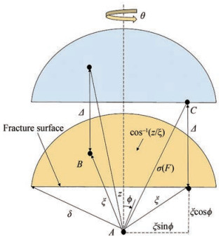Figure  4  Fracture surface with normal opening Δ

Download: Full-Size Img

From Figure 5, we can get s and ξ as follows:

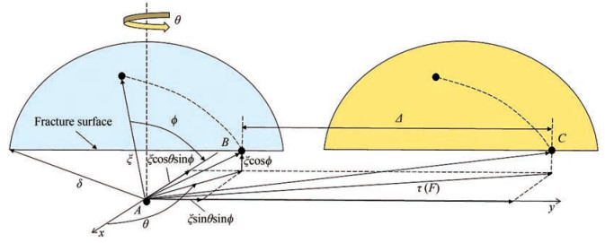Figure  5  Fracture surface with tangential opening Δ

Download: Full-Size Img

The damage will occur when the length exceed ξ, which is depending on s and Δ.

Remark 2.4  We note that in the proposed peridynamics model, both normal and tangential deformation as well as fracture are considered to predict the quasi-brittle failure of ice by using the above established equations.

2.5   Constitutive update

The computational algorithm of the constitutive update or the stress calculation for the ice constitutive model is given as follows:

1. Start to search all material points and initialization parameters;

2. Calculate shape tensor K and inverse;

3. Calculate the approximate deformation gradient $\dot{\boldsymbol{F}} $ and its time derivative;

4. Calculate the spatial velocity gradient L, the deformation rate tensor D, and the asymmetric rotation tensor W;

5. Update the left stretch tensor V and rotate tensor R;

6. Calculate the non-rotational deformation rate tensor d;

7. Select the material constitutive model, and calculate and update the non-rotational Cauchy stress, the von-Mises stress and plastic strain;

(a) Calculate the non-rotational Cauchy stress $\sigma_{n+1}^{\text {trial }} $ of the elastic test;

(b) Calculate the yield function, $ f_{n+1}^{\text {trial }}$, and execute the judgment statement: If $f_{n+1}^{\text {trial }} < 0 $, enter the elastic deformation calculation; If $f_{n+1}^{\text {trial }} \geqslant 0 $, enter the plastic deformation calculation;

(c) Calculate the plastic consistency variable increment Δγ;

(d) Calculate the Cauchy stress;

(e) Update the true equivalent plastic strain;

(f) Output displacement, velocity, acceleration;

8. Calculate the rotational Cauchy stress (true stress), σ;

9. Calculate the first-order Runge-Kutta stress tensor, P;

10. Cycle all material points x_i within the particle neighborhood δ;

11. Calculate the "force state", $\underline{\boldsymbol{T}} $;

12. End loop.

The flowchart of the entire computation of the peridynamics model and the constitutive update for the proposed ice constitutive model are shown in Figure 6.

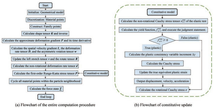Figure  6  Flowchart of the multi-yield surface plastic peridynamics implementation and computation Flowchart of the entire computation procedure Flowchart of constitutive update

Download: Full-Size Img

3   Results and discussions

3.1   Drop tower test

In order to verify the validity and applicability of the proposed ice constitutive model, an ice cylinder is simulated to hit a steel plate at a given impact velocity. The geometrical model size is as shown in Figure 7. The material 1 is chosen to be ice material, and the material 2 is defined as rigid body. There are 74 225 particles and 66 436 cells discrete in total. The mesh size is Δx=1.5 mm, and the horizon size is δ =3.15Δx. Assuming that the cylindrical ice moves at a constant speed, the rigid body does not deform during the collision with the ice body, and the given cylindrical ice provides the conversion of kinetic energy at a certain speed. The calculated material parameters are shown in Table 2.

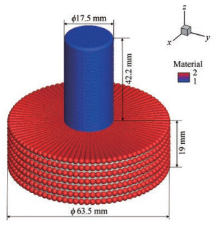Figure  7  Discretized Peridynamic model (Carney et al., 2006)

Download: Full-Size Img

The damage counter of the destruction process of the cylindrical ice with a collision velocity of 152 m/s is shown in Figure 8. The damage factor in the figure is in the range of 0.05−0.95. It can be seen from Figure 8 that the initial damage occurs at the position where the cylindrical ice contacts the cylindrical rigid body, and the ice damage gradually expands upward. Pernas et al. (2012) used three numerical methods: SPH method, ALE method and Largrange method. The predictions of these methods are focused on the deformation of the ice body, and there is no good reflection of the damage and cracks of the ice body. From the calculation results in this paper, it can be seen that the prediction effect of the cylindrical ice damage is that the cracks grow upward from the contact with the rigid body. From 8, the crack propagation and damage process of the cylindrical ice can be clearly shown.

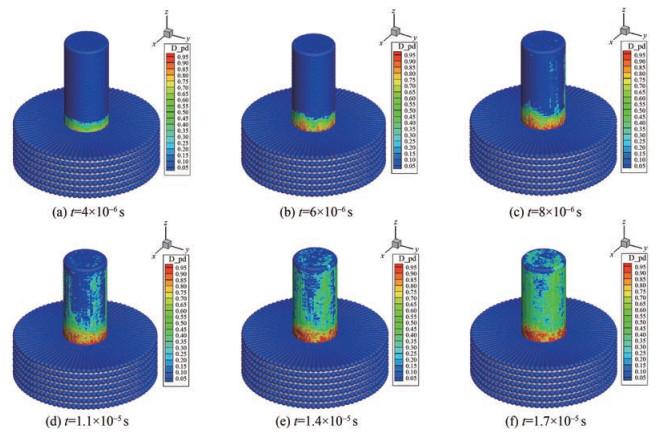Figure  8  Different stages of damage contours of ice at a velocity of 152 m/s

Download: Full-Size Img

Figure 9 illustrates the curve of the collision force between cylindrical ice and rigid body over time. The simulated results are compared with the experimental results of Carney et al. (2006) and the numerical results of (Pernas-Sánchez et al., 2012). The initial speed conditions of 152 m/s and 213 m/s were selected respectively. It can be seen from Figure 9 that the current results is consistent with the experimental results within the time range of 0 ms to 0.1 ms at the initial time (the collision velocity is 152 m/s). The predicted collision force is larger than the experimental one. Before reaching the peak of the collision force, there is a certain forward effect. No elastic deformation occurs when contact occurs, so the calculation result is too large. The collision force reaches its peak at about 0.15 ms, and then gradually decreases as the energy is dissipated. Under the condition of the collision velocity of 213 m/s adopted in Figure 9(b), the calculation results are basically consistent with the experimental results, and the error is smaller than the calculation result of the collision velocity of 152 m/s adopted in Figure 9(a). To a certain extent, the calculation method in this paper is more suitable for high-speed collision conditions, thus verifying the feasibility of the non-ordinary state-based peridynamics constitutive equation used in the calculation of torsional deformation of brittle ice structures. It can be seen from the calculation results of the numerical simulation methods SPH method, ALE method and Largrange method adopted by Pernas that the Peridynamics calculation method used in this paper has certain advantages over other numerical simulation methods.

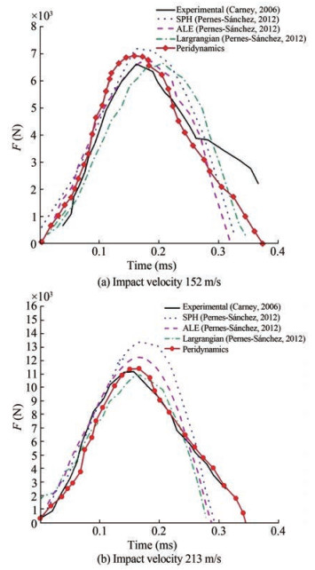Figure  9  The impact force-times curves

Download: Full-Size Img

3.2   Ballistic problem

To investigate the propagation characteristics of ice cracks from the mesoscale perspective, the size of the plate model established here is selected as 0.02 m×0.02 m× 0.001 m thin ice plate, the diameter of the steel ball is 0.001 5 m. A total of 62 203 particles and 50 864 elements are discretized. The rigid ball is assumed to be a rigid body moving at a constant speed, which will not deform during the collision with the ice body. The given rigid ball provides the conversion of kinetic energy at a certain speed. The calculation model is shown in Figure 10. The damage process of ice at a velocity of 150 m/s is shown in Figure 11. The comparison result of the calculated damage contour is shown in Figure 12.

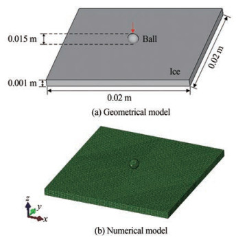Figure  10  Sketch for the ball-ice model

Download: Full-Size Img

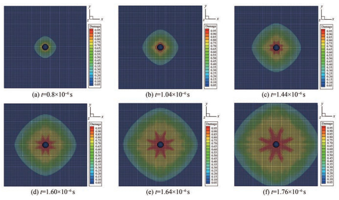Figure  11  Damage process of ice at a velocity of 150 m/s

Download: Full-Size Img

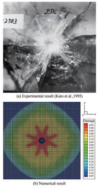Figure  12  Ice fragmentation mode from experiment compared with our numerical result at large view

Download: Full-Size Img

The proposed constitutive has the same effectiveness in processing torsional deformation of ice material. The yield curve equation of the multi-yield surface constitutive model is determined by the parameter constants obtained on the basis of a large number of experiments. It can simulate the plastic deformation of anisotropic materials, and it can simulate the ice failure in the brittle regime as well. Due to the complexity of the structure and composition of the ice material itself, and the different growth and formation processes of the ice, the crystal arrangement is also diverse, so the crack shape of the ice material under high strain rate also presents different manifestations, and has a larger the randomness. This paper selects several experimentally photographed crack shapes during ice breakage from the literature, and compares them with the numerical results in this paper, as shown in Figure 12. In Figure 12, the red area indicates the broken ice body, and the yellow area indicates the ice material in the elasto-plastic stage. Compare with the experimental result, the numerical model can better simulate the crack shape. The crack appears to be broken from the impact center of the ice plate, and the debris area around the center area is approximately circular and runs along the center point, striped cracks radiated all around. The result shows the multi-yield ice constitutive model can better simulate the characteristics of the diversity of ice cracks.

3.3   Ship-ice interaction

In order to verify the applicability of the proposed ice constitutive model in simulating ship-ice interaction, the ice-breaker is used. Assume that the ship is a rigid body and sails through ice at a certain speed. The ship dimensions are chosen in Table 3. The numerical model is built by Abaqus software, and there are 184 225 particles and 126 436 cells discrete in total, as is shown in Figure 13. The mesh size is Δx=1 m, and the horizon size is δ=3.15Δx. Assuming that the icebreaker moves at a constant speed at 5 m/s, the rigid body does not deform during the collision with the ice sheet, and the given ice sheet provides the conversion of kinetic energy at a certain speed. The calculated ice material parameters are the same as Table 2.

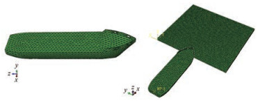Figure  13  Numerical model (Ice breaker)

Download: Full-Size Img

It can be seen from Figures 14‒18 that the proposed method can well capture the dynamic response of the ice, and shows good performance to simulate ship-ice interaction.

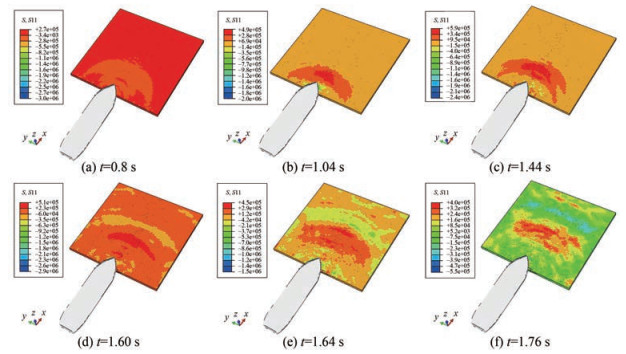Figure  14  Ship-ice interaction process (S11 stress)

Download: Full-Size Img

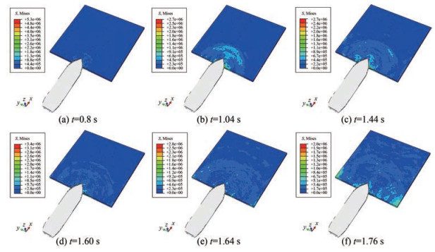Figure  15  Ship-ice interaction process (Von-Mises stress)

Download: Full-Size Img

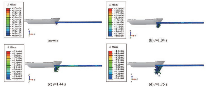Figure  16  Ship-ice interaction process (Damage)

Download: Full-Size Img

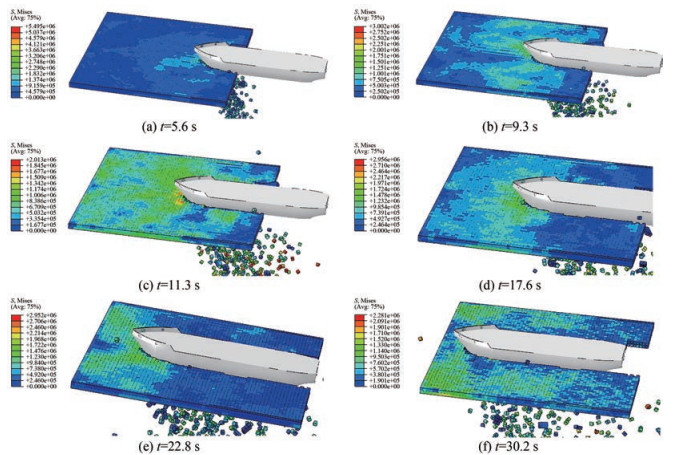Figure  17  Snapshots of a sequence of ship-ice interaction process

Download: Full-Size Img

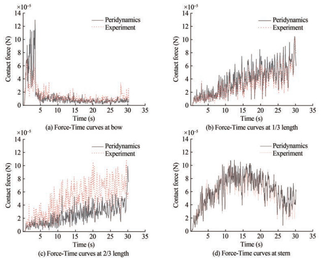Figure  18  Comparison between the peridynamics simulation results and experimental data (Xu et al., 2020)

Download: Full-Size Img

4   Conclusions

In this paper, we developed a state-based cohesive peridynamics model that incorporates a coupled multi-yield surface elastoplasticity model to simulate the stress and crack formation of ice under impact. Compared with the traditional ice constitutive model, the main advantages of the proposed method are:

1) We incorporate the multi yield-surface elastoplasticity model for ice (Derradji, 2002) into the state-based peridynamics formulation, which is then successfully being used to simulate and predict failure of fresh water isotropic ice, iceberg ice, and columnar saline ice.

2) The simulated drop tower test demonstrates that the proposed peridynamics model can better simulate the ice fragmentation under impact loads accurately, and it captures the elastic-plastic quasi-brittle failure behavior in ice, and

3) The proposed method can well capture the ice compressive and tension behaviors in the high strain rate regime, and it shows good performance in simulating shipice collision in ocean engineering applications.

Despite of these advantages, there are still some limitations in the present approach. For example, the influence of the added mass by water is ignored in the present peridynamics model when simulating the ship-ice interaction, and moreover, the ship motion and the subsequent fluidstructure interaction are not considered. Such issues will be addressed in future work.