1   Introduction

The radiated noise of an underwater propulsor affects the comfort of crew members and passengers on a ship and the quietness of a combat vessel. In addition, underwater radiated noise severely affects the navigation, communication, and sensing of some fish and marine mammals, hence affecting their living activities (Hildebrand, 2009). According to the definitions of the Specialist Committee on Hydrodynamic Noise, the underwater radiated noise of ships and underwater vehicles can be classified into hydrodynamic noise, machinery noise, and propulsor noise, where propulsor noise usually dominates the overall underwater radiated noise level of a ship or an underwater vehicle. Consequently, propulsor noise determines detectability and survivability. Understanding the radiated noise characteristics and their relationships with flow, hence reducing the noise of a propulsor, is the ceaselessly pursued goal of researchers in marine engineering. In addition to traditional propulsors, pump-jet propulsor (PJP), as an advanced underwater propulsion system typically consisting of a rotor, a stator, and a duct, has also caught the eye of researchers.

PJP's propulsion performance has been widely investigated through experimental and numerical approaches (Suryanarayana et al., 2010a; 2010b; Shirazi et al., 2019; Wang et al., 2019; Dong et al., 2020). Generally, experimentally obtaining the flow around a propulsor is preferable (Cotroni et al., 2000; Paik et al., 2007; Gong et al., 2022), but the experiment limit is considerable. The flow around a propulsor is usually predicted and studied via numerical approaches (Long et al., 2019; Gong et al., 2018; Li et al., 2020), particularly after the improvement in the numerical method and computing ability. The most employed numerical approach is the method based on viscous computational fluid dynamics (CFD), through which researchers have fully inspected the effects of performance and flow on PJPs and the effects of loading, cavitating, and geometric parameters (Pan et al., 2016; Wang et al., 2020; Yu et al., 2020; Huang et al., 2021; Li et al., 2019). After broadening the view on performance, researchers have devoted themselves to the investigation of flow characteristics to inspect the mechanism responsible for the undesirable characteristics (Ji et al., 2021; Li et al., 2020; Li et al., 2021a; Zhao et al., 2021a; 2021b), hence eliminating or reducing these undesirable characteristics and gaining improvements in efficiency, vibration, or noise.

Although a large number of investigations on the PJP propulsion performance, flow and corresponding prediction methods have been performed, there are few published studies on PJPs concerning noise prediction, the noise generation mechanism, and noise reduction. Sun et al. (2019) utilized the Ffowcs-Williams Hawkings (FW-H) equation together with the sound source obtained by large eddy simulation (LES) to predict PJP noise in effective wake conditions and assessed the effects of serrated trailing edge ducts on noise reduction. Peng and Lu (1998) experimented on PJP noise and determined the frequency spectrum characteristics of the sound pressure level (SPL) curve, showing that the low-frequency spectrum tones are basically the harmonics of the rotor shaft frequency and the blade passing frequency. Zhao et al. (2009) predicted the broadband noise of a PJP via Proudman theory and pointed out that the eddy pulses in the flow field are the dominant factor of noise generation. Fu et al. (2016) predicted PJP noise by the boundary element method based on the theory of point and acoustic fan sources. Xiong et al. (2022) investigated the broadband thrust and loading noise of a PJP under ingested turbulence conditions. The rotor's blade passing frequency (BPF) determines the frequency of haystacking in both the unsteady thrust spectrum and the far-field loading noise spectrum, whereas the dependence of peak frequency on the blade number of the stator is negligible. Moreover, the amplitude and width of haystacking should be related to the ingested turbulent structures.

Some published investigations on PJPs consider the radiated noise performance and noise reduction technology. However, there are still many unknown issues related to the radiated noise characteristics of PJPs, such as the noise characteristics with different primary characteristic parameters (i. e., rotational speed and advance coefficient) and geometry parameters and the effects of cavitating, while for a traditional propeller and ducted propeller, these issues have been properly studied through numerical approaches and even experiments (Wang et al., 2022; Sezen and Kinaci, 2019; Sezen et al., 2021; Ebrahimi et al., 2019; Seol et al., 2002) and have hence broadened the view of noise characteristics of traditional propulsors and, finally, the noise generation mechanism and effective noise reduction technology. In addition, according to the above studies, the FW-H equation is widely used in predicting the noise of underwater propulsors. Combining the FW-H equation with CFD or the potential-based flow solver to predict radiated noise is well known as a hybrid method. Consequently, the spectrum features and overall sound pressure level (OSPL) of a pre-swirl stator PJP with different primary characteristic parameters (i.e., rotational speed and advance coefficient) are systemically and quantitatively considered in this work through the hybrid method. The layout of this article is as follows. After the introduction, Section 2 gives the geometric configuration of the researched PJP, and the numerical method and calculation settings are presented in Section 3. The results and analysis are presented in Section 4. Finally, a summary and conclusions are shown in Section 5.

2   Geometric configuration

The PJP model considered in this work is shown in Figure 1, where the rotor blades and rotor hub are shown in red, the stator blades and stator hub are shown in orange, and the duct is shown in light cyan. The far-field hub is connected with the stator hub through an elliptical guide flow cap. The PJP includes a seven-bladed rotor and a nine-bladed stator. The rotor main parameters are given in Table 1. The radial distribution of the pre-swirl angle of the stator blade, the pitch distribution of the rotor blade, and the duct section coordinates and parameters can be found in Refs. (Li et al., 2021b; 2021c). The rotor rotates around the z-axis, and the rotational direction is right-handed. The rotor diameter is D_r=2R_r=0.166 4 m. The tip clearance between the inside of the duct and the tip face of the rotor is 0.001 m. The PJP was experimented in China Ship Scientific Research Center (CSSRC) to obtain the propulsion performance and wake snapshots. The hydrodynamics and flow field were obtained by a dynamometer and particle image velocimetry (PIV), respectively. Details of the test configuration are shown in Figures 2(c) and (d). The hydrodynamic coefficients are listed as follows:

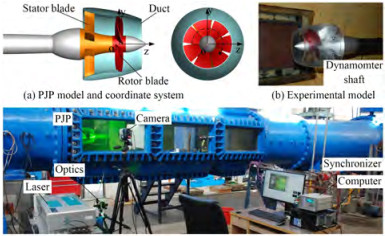Figure  1  PJP model and its experimental configurations

Download: Full-Size Img

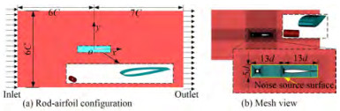Figure  2  Computational domain and mesh of rod-airfoil configuration

Download: Full-Size Img

where J is the advance coefficient and n (r/s) is the rotational speed of the rotor. The rotor period is T_n (s), defined as T_n = 1/n. V_∞ (m/s) is the far-field oncoming flow velocity of the PJP. T_r, T_s, and T_d are the thrusts (N) of the rotor, stator, and duct, respectively, and the corresponding dimensionless forms are K_Tr, K_Ts, and K_Td. The PJP total thrust coefficient is K_T = K_Tr+K_Ts+K_Td. Q_r and Q_s are the torques (N·m) generated by the rotor and stator, respectively. Similarly, their corresponding dimensionless forms are K_Qr and K_Qs. η₀ is the open water efficiency. Unless otherwise specified, all quantities are in dimensionless form handled by D_r, the velocity πnD_r, and the fluid density ρ= 998.2 kg/m³, where the corresponding fluid dynamic viscosity is μ = 0.001 003 kg/(m·s).

3   Computational overview

3.1   Numerical method

In present work, the fluid is regarded as incompressible. The body force and gravitational acceleration are ignored. The Navier-Stokes (NS) equations for the single-phase flow are as follows:

where t is the time. x_i and x_j (i, j = 1, 2, 3) denote the Cartesian coordinates. u_i and u_j are the velocity components, and p is the flow pressure. In most situations, the turbulence described by NS equations cannot resolve the wide range of scales in time and space by direct numerical simulation (DNS) at present. The averaging procedure is applied to the NS equations to filter out all or at least parts of the turbulent spectrum. The Reynolds-averaged procedure applied to the NS equations, resulting in the Reynolds-averaged Navier-Stokes (RANS) approach, is the approach most widely used in obtaining the performances under full wet flow and cavitating flow conditions (Gaggero et al., 2014; Long et al., 2019). The other approach filters the time-dependent Navier-Stokes equations, resulting in the large eddy simulation (LES). Hence, eddies whose scales are smaller than the filter width or grid spacing are effectively filtered out. The resulting equations directly govern the dynamics of large eddies. The large eddy simulation has been employed in resolving the flow around a propeller (Posa et al., 2019; 2020), but there are few cases with ducted propellers and PJPs. The main limits are the geometry and Reynolds number of PJPs being more complex and higher than those of a propeller, respectively. The hybrid RANS/LES approach is a compromise that has been applied in predicting the flow around a propeller (Ji et al., 2012). The most widely used approach in hybrid RANS/LES is the detached eddy simulation (DES) family (Muscari et al., 2013; Long et al., 2021). The RANS portion of the original version of the DES is based on the Spalart-Allmaras (S-A) turbulence model. Then, the RANS portion is extended to the shear stress transport (SST) k- ω turbulence model (Shirazi et al., 2019; Strelets et al., 2001), and the DES has been developed to the improved delayed detached eddy simulation (IDDES) (Gritskevich et al., 2012) step by step. In the DES family, the dissipation term of the turbulent kinetic energy is modified by blending the turbulent length scale. For the IDDES, the blending turbulent length scale l_IDDES is defined as follows:

where l_RANS and l_LES are the turbulent scales of the RANS and LES, respectively. f_d and f_e are the empirical blending function and elevating function, respectively. l_LES is obtained from the LES length scale Δ through a calibration constant C_DES, described as l_LES = C_DESΔ. The LES length scale is defined as Δ = min[C_wmax(d_w, h_max), h_max] where h_max is the grid length scale, d_w is the distance to the nearest wall, and C_w is a model constant. The RANS length scale l_RANS is obtained from the turbulence kinetic energy and specific dissipation rate ω, defined as l_RANS = k^1/2/(C_μω), where C_μ is a model constant. The hybrid RANS/LES (i.e. DES) approach is an alternative approach for obtaining the hydrodynamic sources of noise by utilizing the FW-H or porous FW-H approach (Bosschers et al., 2017). Hence, the IDDES is employed to obtain the flow and sound source in this work.

As revisited in the introduction, the FW-H equation is capable of and widely accepted in calculating the flow noise generated by the flow around underwater propulsors. The FW-H equation is as follows (Ffowcs et al., 1969; Brentner et al., 1998):

where f = 0 denotes a mathematical surface introduced to "embed" the exterior flow problem (f > 0) in an unbounded space. u_n and v_n are the fluid velocity component and surface velocity normal to the surface f = 0, respectively. δ(f) is the Dirac delta function. H(f) is the Heaviside function. p' is the sound pressure. ρ₀ and c₀ are the reference fluid density and sound speed, respectively. The Lighthill stress tensor T_ij is defined as T_ij = ρu_iu_j+P_ij−c₀²(ρ−ρ₀)δ_ij, where P_ij is the compressive stress tensor. As the surface f =0 is not required to coincide with the body surface or walls is permitted as source surface. The sound source of monopole and dipole type are only considered owing to the low flow-velocity. Sound pressure level (SPL) and its overall value (OSPL) of a given frequency range (f_min≤f_i≤f_max) are calculated by following formulas (Sezen and Kinaci, 2019; Wang et al., 2022):

where p' (Pa) is the sound pressure. In this work, the f_max of PJP noise is 2000Hz, larger than the suggested value (Sezen and Kinaci, 2019). For the water medium, the reference sound pressure p'_ref is 10⁻⁶ Pa, and the sound speed is 1 500 m/s.

The noise prediction method is validated using a classic benchmark case (Jacob et al., 2005), not an underwater propeller owing to the lack of experimental noise results of benchmark propellers, the unavailable propeller model, the inconsistent working conditions (cavitating flow and non-cavitating flow), etc. The rod-airfoil configuration is shown in Figure 2. A NACA0012 airfoil (colored in light cyan) with a chord length C=0.1 m is placed downstream of a cylinder (colored in red) with a diameter d=0.01 m, and the main difference from the experiment is the spanwise length. Details of the numerical configuration can be found in Ref. (Chen et al., 2016), where the noise correction method of spanwise difference is also given. More details about the experiment and numerical calculation can be found in Refs. (Jacob et al., 2005; Chen et al., 2016). Here, a permeable surface is adopted as a noise source surface, as shown in Figure 2(b). The noise receiver is located in the middle plane of the airfoil at a distance of 1.85 m. The total number of grids is approximately 4.17×10⁶. The time step is 0.5×10⁻⁵ s, and 5 000 time steps is sampled for noise prediction. The SPL curve at the preset receiver is shown in Figure 3. The numerical prediction obtains the tonal peak, but the broadband components are higher than those of the experiment, showing results similar to those of Ref. (Chen et al., 2016). Overall, the radiated noise predicted by using the IDDES and FW-H is feasible.

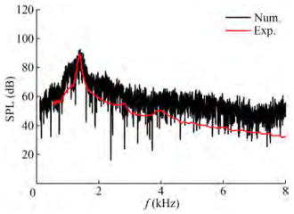Figure  3  SPL curve at the receiver

Download: Full-Size Img

3.2   Calculation settings

The computational domain is a cylinder with the PJP located in the centerline. Details are shown in Figure 4. The PJP and its near field are enclosed by a cylindrical subdomain, named outer domain 0 and the exterior part of outer domain 0 is the far-field, named outer domain 1. In the PJP inner passage, the stator and rotor are also enclosed by subdomains, named the stator and rotor domains, respectively. The subdomains are connected through interfaces. The computational domain is discretized by structural mesh as the blade cascade is convenient for generating structural girds. Figure 5 presents the mesh on the PJP surface and flow field. The mesh of the near field and the PJP wake region, particularly the duct trailing edge downstream, are refined. The blade tip region is also refined. To ensure the wall y+ is close to or lower than 1 for the IDDES calculation, the first layer heights of the normal wall mesh are 3×10⁻⁶ m for rotor blade surfaces and 5×10⁻⁶ m for the rest of the wall surface. Three mesh groups are generated to assess the effects of mesh density on the prediction of propulsion performance, successively named G1, G2, and G3. The total grid numbers of the G1, G2, and G3 mesh groups are 4.44×10⁶, 10.19×10⁶, and 23.01×10⁶, respectively.

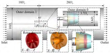Figure  4  Divided subdomains and boundary conditions

Download: Full-Size Img

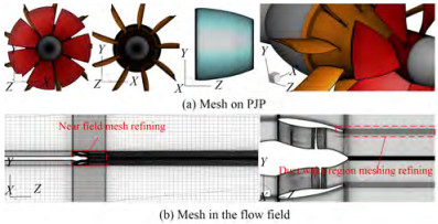Figure  5  Mesh views of the PJP surface and the flow field

Download: Full-Size Img

The inlet of the computational domain is a velocity inlet. When varying the advance coefficient, the rotational speed of the rotor is fixed at n = 20 r/s, and then, the V_∞ value is determined. The advance coefficient ranges from 0.2 to 1.2 with a step size of 0.2. When varying the rotational speed of the rotor, the advance coefficient is fixed at J = 1.0, and then, the V_∞ value is determined, where n ranges from 10 to 30 with a step size of 5. The values of the turbulence intensity and turbulence viscosity ratio in the inlet are set to 1% and 10, respectively. The computational domain outlet is a constant-static pressure outlet with a value of 0. The shear stresses on the lateral cylindrical wall of the computational domain are set to zero. The effects of mesh density are only considered in steady RANS calculations, which has been discussed in many previous investigations. In the IDDES, the time step size is set according to the rotor rotational speed, defined as Δt = 1/(360n). In addition, the effects of the time step have also been discussed in many previous PJP investigations(Li et al., 2020; 2021a; Ji et al., 2021), which indicates that the present time size is sufficient for predicting propulsion performance and flow details. Before obtaining the noise source, calculation sustains eight times the rotor periods for a statistically stable flow field. The time of obtaining the noise source are 22 times period of the rotor. Hence, the sampling time is larger than 1 s. Consequently, the frequency resolution of the sound pressure in the frequency domain is less than 1 Hz. The interface that encloses outer domain 0 is set as the source surface.

As shown in Figure 4, outer domain 0 is a cylinder with a length of L_0d = 3.7D_r and a diameter of 1.6D_r. In addition, the effects of different lengths of outer domain 0 on noise prediction are considered. For all calculations, the SIMPLEC algorithm is employed. In the RANS steady calculation, a second-order upwind scheme is used to discretize the momentum equations and the k and ω equations. In the IDDES, the momentum equation and time term are discretized by the bounded central differencing scheme and bounded second-order implicit scheme, respectively. All calculations are performed by the Fluent double precision solver. The noise receivers are shown in Figure 6, where R is the distance between the PJP and receiver. The receivers in the yOz and xOy planes are differentiated using subscripts. The source SPL(R = 1 m) is calculated based on the noise reduction law in the free sound field.

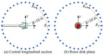Figure  6  Locations of the noise receivers

Download: Full-Size Img

3.3   Comparison with experiment

The steady RANS results and IDDES results of propulsion performance are shown in Figure 7, where the stator torque is the absolute value. The effects of mesh density on the propulsion calculation are assessed based on the theory of grid convergence (Celik et al., 2008), and the results are given in Table 2. According to the grid convergence index (GCI), the mesh density is sufficient for a better performance prediction. The IDDES results show good agreement with the experiment.

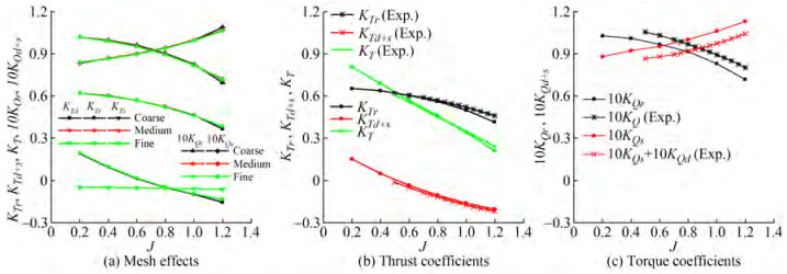Figure  7  Open water performance obtained by the RANS and IDDES and their comparison with the experiment

Download: Full-Size Img

At J = 0.8, the distributions of velocity components in the z and y directions on the central longitudinal section (yOz plane) are presented in Figure 8, where the region z ≤ 0.4D_r of the PIV is affected by the duct in the experiment, so there is no data. For a qualitative point, the numerical results are acceptable compared with the experiment, including the hub wake region and the buffer region between the free stream and high-velocity core of the wake. The velocity component in the z direction V_z in the yOz plane at the axial positions z = 1.0D_r and 1.5 D_r are exhibited in Figure 9. The velocity distribution trend along the y direction is well captured. Overall, the IDDES turbulence modeling approach is able to obtain the flow around the PJP.

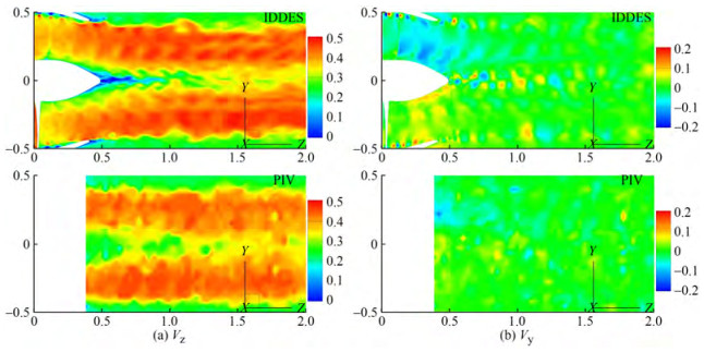Figure  8  Distributions of V_z and V_y in the yOz plane at J=0.8

Download: Full-Size Img

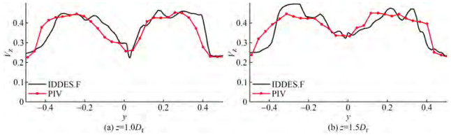Figure  9  V_z at the axial locations in the yOz plane

Download: Full-Size Img

The sound pressure is a very small value compared with the flow pressure. To assess the underlying numerical error caused by the limited precision, the effects of the precision level are given in Figure 10(a), where f_BPF is the blade passing frequency, defined as the product of the rotor blade number and rotor axis frequency (f_n equals to the rotational speed). The precision shortage results in a loss of tonal noise and higher broadband noise. According to the previous investigations on PJPs (Peng and Lu, 1998) and propellers (Sezen et al., 2019), the radiated noise generated by rotational blades has noticeable tonal noise with dominant values (not only higher than the broadband components but also larger than most of the other tonal components). Consequently, it requires a higher-precision solver to obtain the sound source. As shown in Figure 4, the sound source has a length of L_0d = 3.7D_r and a diameter of 1.6D_r. The length L_0d affects the size of the PJP wake included in the sound source. As shown in Figure 10(b), the increased inclusion of the PJP wake has notable effects on both the tonal noise and broadband noise. A small source region results in considerable reductions in broadband noise and a loss of the tonal peaks at typical frequencies. In addition, the sampling frequency affects the capture of tonal peaks, including the value of the peak and the location, as depicted in Figure 10(c). A small enough sampling frequency is preferable. In this work, the sound source is obtained by a double-precision solver in the sound source region with an axial length of L_0d = 3.7D_r. The sampling frequency is lower than 1 Hz for a better capture of the tonal noise. In addition, only the noise contribution in the frequencies ranging from 0 to 2 000 Hz to the OSPL is considered.

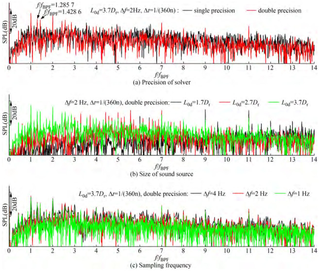Figure  10  Effects of computational setting during noise prediction

Download: Full-Size Img

4   Analysis and discusion

4.1   Performance

The effects of the rotor rotational speed on PJP performance are presented in Figure 11. With the same advance coefficient, the rotational speed affects the Reynolds number and, hence, the flow on the PJP. Like a propeller, the performances of the model scale PJP change with different rotational speeds. Particularly, the torque of the stator has a noticeable deviation between the highest and lowest rotational speeds. The rotor thrust also shows increased deviation as the advance coefficient increases. Although the thrust changes of the rotor, stator, and duct are not very noticeable at different rotational speeds, the total thrust of the PJP shows a noticeable deviation because the thrust trends are the same. Sometimes, the rotational speed is important for a model scale propulsor. At the same advance coefficient, it should be ensured that the blade works above the critical Reynolds number. If the rotational speed cannot adopt a high value, the flow transition of a propulsor model should be considered. Nevertheless, the flow transition will complicate the numerical prediction and might cause a more significant deviation from the full-scale model.

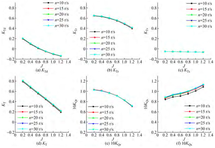Figure  11  Open water curves under different rotational speeds

Download: Full-Size Img

The thrust fluctuations of the rotor with different advance coefficients and different rotational speeds are shown in Figure 12, where σ_rotor is the root mean square value of the thrust fluctuation. The rotor shows a significant thrust fluctuation at the lowest advance coefficient (J = 0.2). At J = 0.4, the thrust fluctuation level notably decreased from 0.352 5% to 0.097 9%. With the advance coefficient continuously increasing, the degree of thrust fluctuation decreases but increases at the advance coefficient J = 1.2. According to previous investigations, the aggravation of thrust fluctuation is caused by flow separation on the duct, and meanwhile, the inflow of the rotor is more nonuniform and hence the higher fluctuation. At the same advance coefficient (here, J = 1.0), the thrust fluctuation changes slightly and shows a varying trend of decreasing first and then increasing with increasing rotational speed.

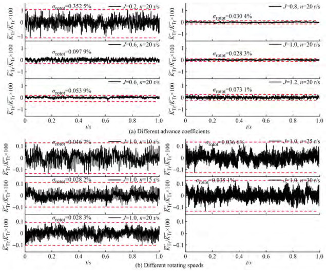Figure  12  Thrust fluctuation of the rotor

Download: Full-Size Img

The thrust fluctuation is transformed into the frequency domain as shown in Figure 13. In the frequency domain, the thrust fluctuation presents noticeable peaks at the frequencies of f_BPF and harmonics of f_BPF. There are also many peaks that are not at f_BPF and its harmonics. The peak at frequency f/f_BPF = 1.285 7 is also noticeable, and this frequency value is equal to the product of the axis frequency and stator blade number, here defined as f_s. At J = 1.2, there is a peak at frequency f/f_BPF =2.285 7, which equals the sum of f_BPF and f_s. Tonal peaks are located at not only f_BPF and f_s but also their harmonics. There are also many peaks whose frequencies are not equal to the harmonics of f_BPF, the harmonics of f_s, or the harmonics of f_n when the PJP works at the heaviest or the lightest load. According to previous investigations, those peaks are caused by flow separation on the duct.

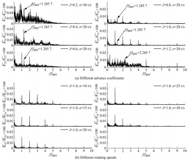Figure  13  Frequency-domain curves of the thrust fluctuation of the rotor

Download: Full-Size Img

Unlike changing the advance coefficient, varying the rotational speed mainly affects the amplitudes of peaks at f_BPF and f_s, and their harmonics. At n = 10 r/s and 15 r/s, the maximum amplitude is located at 2f_BPF. As the rotational speed increases, the maximum amplitude peak shifts to f_BPF. The high-order harmonics of f_BPF decrease considerably. From the thrust fluctuation both in the time- and frequency-domains, a high rotational speed of the rotor in the model during the numerical prediction and experiment is preferable for obtaining a more similar performance and more reliable degree and dominant frequency of thrust fluctuation.

4.2   Radiated noise

Figure 14 shows the radiated noise of receiver R₁ when J = 1.0 and n = 20 r/s. The SPL curve consists of tonal components and broadband components, where some tonal components have considerable amplitudes. These dominant peaks are located at f_BPF and at the harmonics of f_BPF. The peak at 1.285 7 f_BPF is the stator blade passing frequency f_s. The peak at 1.428 6f_BPF is the harmonics of f_n, equal to 10f_n. At 4f_BPF, 5f_BPF, 7f_BPF, and 9f_BPF, the peaks are also visible, but they have relatively small amplitudes. The SPL curves of different receivers when J = 1.0 and n = 20 r/s are shown in Figure 15. This six receivers are located at the three axes, where R₁ and R₁₉ are located on the z-axis, R₁₀ and R₂₈ are located on the y-axis, and R₃₇ and R₅₅ are located on the x-axis. This demonstrates that the abovementioned dominant peaks do not change at different receivers, while the peaks at other harmonics of f_BPF show obvious differences, such as the peaks at 4f_BPF, 5f_BPF and 9f_BPF. In addition, the broadband noise level also has a difference in the frequency band 7f_BPF ≤ f ≤ 10f_BPF. Overall, the SPL curves are highly consistent.

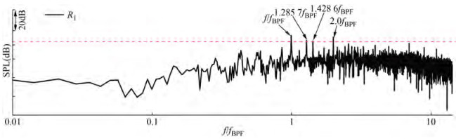Figure  14  SPL curve of R₁ (J=1.0, n=20 r/s)

Download: Full-Size Img

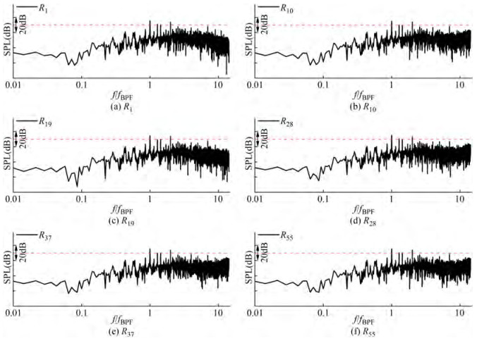Figure  15  SPL curves of different receivers (J=1.0, n=20 r/s)

Download: Full-Size Img

Based on the preset receivers, the directivity of the source OSPL is shown in Figure 16. In the yOz plane, the noise in the y direction is larger than that in the z direction, where the difference of the two extreme OSPL values in the z and y directions is up to 2.42 dB. The OSPL curve presents an "ellipse" shape, indicating that the PJP has a higher radiated noise level in the side directions and obvious directivity. In the xOy plane, the OSPL curve is almost a "circle" shape and the difference of the two extreme OSPL values is 0.14 dB, demonstrating a slight directivity or almost no directivity.

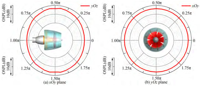Figure  16  Directivities of the OSPL in the yOz and xOy planes (J=1.0, n=20 r/s)

Download: Full-Size Img

When fixing the rotational speed and varying the advance coefficient, the SPL curves present noticeable changes in both tonal noise and broadband noise, as depicted in Figure 17. The number of tonal peaks increases with increasing the advance coefficient, while the broadband noise decreases first and then increases above J = 1.0. In the low advance coefficients J = 0.2, 0.4, and 0.6, the tonal peaks almost disappear, and the broadband noise increases considerably in the frequency band 0≤ f ≤7f_BPF. At J = 0.8, a dominant tonal peak occurs at 2f_BPF. When the advance coefficient increases to 1.0 or 1.2, not only the frequency at f_BPF, f_s but also the frequencies of their harmonics show dominant values. The broadband component also increases at the highest advance coefficient, which is highly related to the flow separation on the outside of the duct.

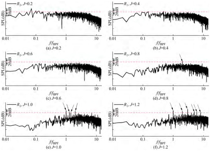Figure  17  SPL curve for receiver R₁ when varying the advance coefficient

Download: Full-Size Img

The directivities of the source OSPL in the yOz and xOy planes at different advance coefficients are given in Figure 18. The OSPL shows a decreasing trend versus the advance coefficient, but from J = 1.0 to J = 1.2, the OSPL increases. This is highly dependent on the increased broadband noise and more dominant tonal peaks. In the yOz plane, the OSPL shows a larger value in the side directions and the directivity becomes notable as the advance coefficient increases. From J = 0.2 to 1.2, the differences of the two extreme OSPL values are 0.82 dB, 0.84 dB, 0.97 dB, 1.34 dB, 2.42 dB, and 3.29 dB, respectively. However, the differences of the two extreme OSPL values in the xOy plane from J = 0.2 to 1.2 are 0.02 dB, 0.02 dB, 0.04 dB, 0.08 dB, 0.14 dB, and 0.10 dB, respectively. The directivity in the xOy plane does not show any notable change. The directivity is still very slight.

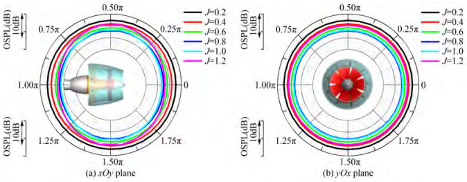Figure  18  Directivities of the source OSPL when varying the advance coefficient

Download: Full-Size Img

When considering the effects of rotational speed, the SPL curve shows noticeable changes in tonal components, which is different from that of the thrust fluctuation spectrum of the rotor. As shown in Figure 19, a higher rotational speed of the rotor results in more abundant and higher tonal peaks and larger broadband noise. The SPL curve only shows a notable peak at f_BPF when J = 1.0 and n = 10 r/s. When the rotational speed increases to 15 r/s, the tonal peaks becomes more abundant, not only at f_BPF and f_s but also at the harmonics of f_BPF, f_s, and f_n. Changing the rotational speed causes a higher noise level and considerable differences in the noise spectrum.

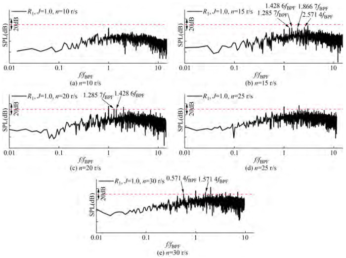Figure  19  SPL curve of R₁ when varying the rotational speed

Download: Full-Size Img

The directivity of the source OSPL with different rotational speeds is shown in Figure 20. Increasing the rotational speed does not change the directivity of source noise in the xOy plane but causes notable directivity differences in the yOz plane. In yOz plane, as the rotational speed increases, the differences of the two extreme OSPL values in the yOz plane are 0.91 dB, 2.92 dB, 2.42 dB, 1.85 dB, and 1.07 dB, respectively. The directivity becomes notable first and then slight. Comparatively, the differences in the xOy plane are 0.05 dB, 0.06 dB, 0.14 dB, 0.17 dB, and 0.09 dB, indicating a slight directivity change. The varying trend of radiated noise at R₁ with the advance coefficient and rotational speed are shown in Figure 21. Though varying both the advance coefficient and varying rotational speed results in notable differences in the noise spectrum, the OSPL of radiated noise at the far-field receiver shows a difference in varying trends. With increasing the advance coefficient, the OSPL decreases and then increases, and the varying degree is small while it shows a considerable increasing trend with increasing the rotational speed of the rotor. To achieve a low OSPL, decreasing the rotational speed of the PJP rotor is the first choice.

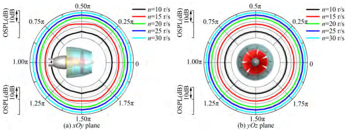Figure  20  Directivities of the source OSPL when varying the rotational speed at J=1.0

Download: Full-Size Img

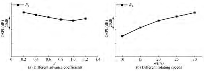Figure  21  OSPL of R₁ under the effects of advance coefficent and rotational speed

Download: Full-Size Img

5   Conclusion

The present investigation shows the capabilities of the IDDES based on a sufficient mesh density in resolving the flow around the PJP and obtaining the flow noise source. The porous FW-H equation is adopted to calculate the far-field noise signals. After discussing the performance and thrust fluctuation under different advance coefficients and different rotational speeds, the radiated noise characteristics of the PJP are analyzed. Some important observations are drawn as follows.

The propulsion performance shows some minor deviations as the flows around the rotor, stator, and duct are not completely similar under different operating conditions. In addition, the flow differences notably affect the fluctuation characteristics of rotor thrust, including the degree and spectrum. The distribution and amplitude of spectrum are largely determined by the advance coefficient, but the effects of rotational speed cannot be ignored, such as the frequency shift of dominant peaks.

The radiated noise characteristics of the PJP are highly affected by both the advance coefficient and rotational speed of the rotor, including the distribution tonal noise and the level of broadband noise. A higher advance coefficient results in multiple tonal noises but a lower intensity of broadband noise. At the same advance coefficient, a high rotational speed of the rotor causes not only more abundant high tonal noise but also high broadband noise. The OSPL is highly determined by the rotational speed. When the rotational speed is fixed, larger loading on the PJP results a higher OSPL, but the increment is small. However, the OSPL shows an inverse increase when the load is very light. This is highly related to flow separation on the PJP. The directivity of the source OSPL in the side direction plane is highly affected by the advance coefficient, not the rotational speed of the rotor. The directivity is gradually enhanced as the advance coefficient increases. In the axial direction plane, the directivity is almost negligible and is not affected by the advance coefficient or rotational speed.

Although the radiated noise characteristics with different advance coefficients and rotational speeds are obtained, some conclusions of the overall SPL are only applicable to frequency bands below 2 000 Hz. In future work, more deep investigations and model experiments will be carried out to assess the effects of the rest of the frequency band.