1   Introduction

Duplex stainless steel exhibits high strength and excellent stress corrosion resistance, which are suitable for marine engineering (Chen et al., 2022). Additive manufacturing (AM) is a 3D solid rapidly available manufacturing technology and is one of the key development implications for future innovation. Wire and Arc Additive Manufacture (WAAM) adopts layer-by-layer surfacing to manufacture dense metallic solid parts. Owing to its high heat input and fast forming speed, it is suitable for the low-cost, efficient, and fast near-net shape formation of large and complex components. This technology has incomparable efficiency and cost advantages over other additive technologies in manufacturing large-sized structural parts. The combination of WAAM and marine manufacturing is a hot topic in marine manufacturing. WAAM can be used for the direct formation of large ship parts and is especially suitable for the on-site repair of ship parts. Many studies have been conducted on the welding of duplex stainless steel (Landowski et al., 2020; Maurya et al., 2021; Świerczyńska et al., 2020; Maurya et al., 2022a; Maurya et al., 2022b), but only a few have focused on the WAAM of duplex stainless steel. In the present work, the WAAM of duplex stainless steel using tungsten inert gas-shielded welding was carried out, and the quality of weld bead formed using duplex stainless steel was predicted. The results can provide scientific guidance for the WAAM of duplex stainless steel components.

Gas-shielded tungsten inert welding (TIG) (Moreira et al., 2020) is one of the widely used welding heat sources and has the characteristics of stable arc, no reaction between shielding gas and metal, convenience, and flexibility (Ayarkwa et al., 2017). WAAM is based on the stacking of overlapping weld beads, and the quality of weld beads directly affects the quality of the processed workpiece (Sahoo et al., 2021). Given that the welding process is nonlinear, multivariable, and complex, the weld quality is directly related to the welding process (Durga et al., 2021). Guo et al. (2018) found that when welding 5083 aluminum alloy with molten electrode plasma arc, an increase in welding current and a decrease in welding speed (WS) increase the depth of melt. When conditions such as 230 A current, 0.9 m/min wire feed speed, and 6.5 L/min shielding gas flow rate are adopted, the maximum tensile strength of the welding area reaches 274 MPa, which is close to 86% of the base material. Le et al. (2021) found that the optimal process parameters for the arc augmentation of 308L stainless steel wire are 368 mm/min wire feed speed, 22 V welding voltage, and 122 A welding current, which can obtain a single-layer single-pass with a smooth and regular surface, reduce heat input, and ensure the stability and quality of 308L walls. Owing to the different melting points of different kinds of metal wires, such as ER5356 (Yuan et al., 2020), ER2319 (Qi et al., 2019), and 316L (Wang et al., 2022), their suitable WAAM process parameters also vary. The welding currents of the above welding wire materials are 90 – 110, 120, and 150 A, respectively, and their wire feeding and WSs are different. Variations in thermal expansion coefficient and deformation behavior are found between austenite and ferrite in duplex stainless steel. The inharmonious deformation of the two phases is prone to the formation of edge cracks (Zhao et al., 2019), resulting in a complex welding process of duplex stainless steel (Martins and Casteletti 2009). Many complex factors influence weld bead quality and bring great challenges to the accurate prediction of weld quality (Martina et al., 2019; Sasikumar et al., 2021). Therefore, studying the effect of process parameters on the dimensions of duplex stainless steel formed by WAAM is of great significance to realize the accurate prediction of weld quality.

With the rapid development of artificial intelligence, algorithms that establish mathematical models to predict the objective function have been applied in the field of welding. Wang et al. (2021) used the vision sensing system to collect weld pool images during welding and proposed an active interference suppression control algorithm based on deep learning that provides the necessary strategy for the online monitoring and control of weld width during WAAM. To reduce the offset of the deposited layer in WAAM, He et al. (2021) used the depth residual network to predict the deposited layer offset according to the visual morphology of the melt pool obtained by the vision sensor and found that the average prediction error is less than 0.14 mm. Xue et al. (2018) established a back-propagation (BP) neural network to predict WAAM weld bead geometry, but the prediction results are not ideal due to the presence of many process parameters and model output parameters. Tian et al. (2013) developed a TIG weld size prediction model based on a genetic algorithm to optimize the BP neural network and obtained the optimal solution method for the weights and threshold values of the BP neural network that produces good prediction results (Xiao et al., 2009; Yi et al., 2007). Particle swarm optimization (PSO) is an iteration-based optimization algorithm that is easy to implement and does not require the adjustment of many parameters. It is superior to traditional optimization algorithms (such as genetic algorithms) and is often used to optimize models to find the optimal solution. Kumar et al. (2020) used PSO and multiobjective optimization to obtain the best process parameters for the best joint quality. To predict weld bead morphology, Liu (2020) proposed a nonlinear fitting image analysis system based on image processing and mathematical function models. The relationship between welding process parameters and single-layer forming dimensions, welding process parameters, and multipass forming dimensions was established. Ding et al. (2015) and Cao et al. (2010) proposed three single-layer single-pass weld cross-sectional function models with circular arc function, cosine function, and curved function to achieve the fitting and prediction accuracy of weld cross-sectional sizes when multilayers and multipasses overlap.

Although the predictions of different weld bead dimensions and real-time error monitoring of WAAM sizes are available, all these methods require high-cost equipment and complex mathematical models. This study mainly adopted the BP neural network algorithm (Ghafarallahi et al., 2021), which has strong nonlinear mapping capability and flexible network structure but slow learning speed and is prone to falling into local minima. PSO can effectively compensate for the shortcomings of BP neural networks by seeking individual optima via the initialized random particles, sharing the position with the overall particle swarm, and finally finding the global optimum value, thus improving the prediction accuracy and generalization ability of the model. Therefore, this study used the PSO-optimized BP (PSO-BP) neural network algorithm to accurately predict the weld bead formation of duplex stainless steel WAAM. This approach can be applied to predict the process parameters required for single-pass welding wire and can also provide single-pass size prediction for the repair of large duplex stainless steel parts (i.e., corroded or worn ship hull, large gear, and propeller) to reduce actual repair errors and defects. In addition, this study provides a new idea for the research of lap ratio and path planning of large and complex parts manufactured by arc additives.

ER2209 duplex stainless steel wire manufactured by WAAM was selected as the experiment object, and the response surface methodology was used to optimize the TIG WAAM process parameters. The effects of welding current, WS, wire feed speed, and their interaction on the weld bead width and height were analyzed. The weld bead size prediction models of BP and BP-PSO were established with MATLAB software, and their prediction results were compared. Finally, the fitting function of the weld bead cross-sectional shape was applied to lay the groundwork for the exploration of duplex stainless steel multiple weld bead formation. The remainder of this article is organized as follows. Section 2 introduces the experimental methods, Section 3 presents the results and discussion, and Section 4 shows the main conclusions.

2   Experiment

2.1   WAAM and materials

As shown in Figure 1, the trial was carried out on a self-built automatic TIG WAAM platform made up of a KUKA model KR 60 HA machine arm, a Shenzhen Ruiling YC-315 TIG welder, and a WF-007A wire feeder. Ar₂ with a purity of 99.99% was used as the protective gas.

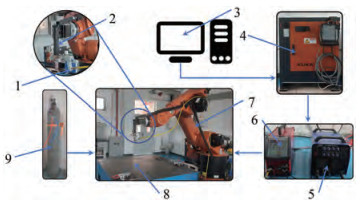Figure  1  WAAM test platform

1: Wire feed nozzle; 2: TIG torch; 3: Computer; 4: Control cabinet; 5: YC-315 electric welder; 6: WF-007A wire feeder; 7: KUKA KR 60 HA robot arm; 8: Mild steel table; 9: Argon shield gas

Download: Full-Size Img

2.2   One-factor and response surface experiments

First, the effects of wire feeding speed (WFS), WS, and welding current on the formed bead size of duplex stainless steel were studied. The other parameters were set to fixed values, including argon shielding gas flow rate of 15 L/min, tungsten electrode extension of 3 mm, and wire feeding angle of 30°. Suzhou EDM wire cutter model M340 was used to cut the formed single-layer weld to obtain the cross-sectional profile of the bead. The section was observed with a high-precision OPLENIC metallurgical microscope and measured with EZcam software to obtain the microstructure, melt width, and height of the bead. Figure 2 shows the overall flow diagram of this study.

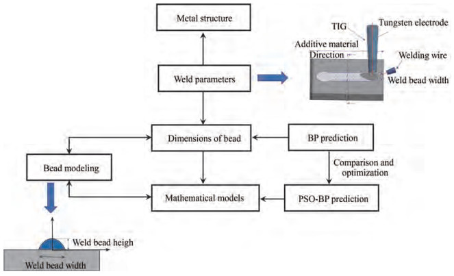Figure  2  Flow block diagram

Download: Full-Size Img

From the single-factor response surface experiment, the weld bead width and height were taken as the evaluation criteria of formed weld bead quality. The influence law and interaction of each parameter on weld bead width and height were studied. The weld bead width and height were taken as response values. A response surface analysis test table with three factors and three levels was designed in accordance with Box – Benhnken central combination test theory, as shown in Table 1. Various process parameters were designed according to the surface response method, and the measurement results of weld bead size were recorded. The correlations of weld bead width and height with wire feed speed, WS, and welding current were verified.

2.3   PSO-BP neural network model

BP neural network is a multilayer feedforward neural network with forward signal propagation and using an error back-propagation algorithm as the correction training algorithm. This method is simple and practical and is one of the most commonly used approaches to study and predict the process parameters of welding seam (Qi et al., 2019; Wang et al., 2022; Zhao et al., 2019; Martins et al., 2009). BP neural network is a typical neural network composed of three or more layers of neurons. The structural direction is from left to right, and the neurons are connected by weights between the layers. The gradient of the loss function relative to each neuron is calculated, and the weight is updated in the process of gradient BP error and iterated continuously until convergence.

The weight iteration formula is as follows:

where ∆ω_ij (n) is the difference of the n_th iteration weight, and E denotes the mean square error of the output layer. The first term is the conventional learning factor term, which is the learning factor that can be set based on the specific situation, and the second term is the momentum term, which is the momentum factor. The sample data must be normalized to remove the effect of dimensionality between indicators before running the network algorithm.

where X represents the value after data normalization, X∈ [−1, +1], and max/min (A) represents the maximum number of data elements in the same column. A is all the elements of the same column, and x is the value of a specific digit on that column. BP neural network implements an input-to-output mapping function. The mathematical theory has demonstrated that three-layer neural networks can approximate nonlinear continuous functions with arbitrary accuracy. The following empirical formula is used as a general reference:

where n is the number of neurons in the input layer, m is neurons in the output layer, a∈[1,10], and l is the number of neurons in the hidden layer. In this study, the welding current, WS, and wire feed speed parameters were selected as the neurons of the network input layer, and the height and width of the weld bead were selected as the neurons of the output layer. According to the calculation results of the error value of the performance function under different hidden layers, the neural network prediction model has a 3-12-2 structure, as shown in Figure 3.

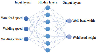Figure  3  BP neural network structure

Download: Full-Size Img

PSO is a population intelligence algorithm based on the study of the predatory behavior of birds or fish. The basic idea is to assume that a certain number of particles are initialized to simulate birds in a bird swarm. Each particle has two attributes: velocity and position. The velocity of the particle determines the direction and distance and is dynamically adjusted according to the flying experience of the particle and its partners. The particles track these two extremum optimization updates through the given memory function and continue to iterate until the group optimal solution is found. The D-dimensional space is made up of N randomly initialized particles, and particle i position is X_i = (x_i1, x_i2, …, x_iD), X_i substitute into the adaptation function f (X_i) to find the adaptation value. The velocity of particle i is W_i = (v_i1, v_i2, …, v_iD), the individual extrema of particle search are denoted by P_i = (p_i1, p_i2, …, p_iD), and the particle population search's global extreme point is defined by g_i = (g_i1, g_i2, …, g_iD).Following the search for the individual and global extremes, the particle velocity and position update equations are as follows:

where V_iD^k and X_iD^k denote the D_th dimensional components of the velocity vector and position vector of particle i's flight in the k_th iteration, respectively; c₁ and c₂ are the learning factors; r₁ and r₂ are two random variables in the range [0,1]; and W is inertial weight adjustable spatial search range. A linear decreasing strategy with the following formula is usually used to enhance PSO's global and local convergence capability to find the best solution.

where w_i(t), w_ini, w_end, and G denote the weight of the t_th iteration, the initial weight, the termination weight, and the total number of iterations, respectively. Weights and thresholds are assigned at random in the simple BP neural network structure, and the PSO algorithm optimizes the BP neural network mainly by treating the weights and thresholds as particles. Figure 4 shows the flow chart for developing the PSO-BP prediction model.

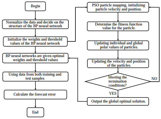Figure  4  PSO-BP prediction model flow chart

Download: Full-Size Img

In this work, 87 groups of tests with various process parameters were carried out. Among these, 57 groups of data were chosen as training samples, and the rest were used as test samples for prediction. The training process ended when the training error as an index reached a constant or specified minimum value. The data obtained from the response surface test were divided into training and testing data. All selected data samples were then normalized, and the topology of 3-12-1 was selected on the basis of the above parameters for the BP model. Tansig was chosen as the signal conditioning for the implicit layer and Purelin for the output layer. The training time was set to 1000, the learning rate was 0.1, and the expected error was 10^{− 5}. The above parameter settings were substituted into MATLAB language programming to obtain the training results. PSO was also used to optimize the BP neural network for prediction. Finally, the experimental results, BP neural network prediction, and PSO-BP neural network prediction were compared.

2.4   Determination of the fitting function for the weld bead section

The weld bead profile image was processed by a 3D scanner to generate an STL file, and then the average cross-sectional profile of the weld bead was calculated by MATLAB image processing. The coordinates of two points at the bottom and one point at the top of the profile were determined, and different model functions were used for fitting. The mean square error ratio of different models was calculated. After comparison with the fitting accuracy of different models, the optimal fitting function model was determined.

3   Results and discussion

3.1   Effect of WAAM process parameters on weld bead forming dimensions

3.1.1   Width of weld beads

Figure 5 shows the effect of wire feed speed, WS and welding current on the width of the weld bead. The upper and lower bars in the figure represent the fitted error limits. As shown in Figure 5a, the weld bead width increases with the wire feed speed. The reason is that when the heat input, welding current, and WS are constant, the wire feed speed and the amount of wire melt increase, resulting in an increase in bead width. Figure 5b shows that the bead width decreases significantly with the increase in the WS because of the reduced amount of cladding per unit time. Figure 5c shows that the weld bead width increases linearly with the welding current. The reasons are that when the current increases, the diameter of the arc melt pool and the heat also increase, and the corresponding weld bead width becomes widened.

Figure  5  Effect of WAAM process parameters on weld bead width

Download: Full-Size Img

3.1.2   Height of weld bead

Figure 6 shows the effect of WAAM process parameters on weld bead height. As displayed in Figure 6a, the bead height increases with the wire feed speed. The reason is that when the heat of the molten pool is constant, the increase in the wire feed speed causes the unmelted welding wire to absorb heat. Hence, the bead height increases with the cladding amount. Figures 6b and 6c show that the bead height approximately linearly decreases with the increase in WS and current. The first reason is that when the heat output of the molten pool remains constant, the WS increases, and the cladding amount per unit time decreases. Thus, the bead height decreases. The second reason is that when the wire feed speed and WS remain constant, that is, when the cladding amount remains constant, the welding current and heat output increase. Thus, the bead height decreases.

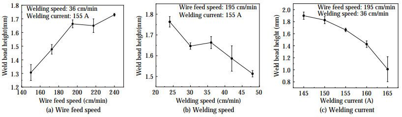Figure  6  Effect of WAAM process parameters on weld bead height

Download: Full-Size Img

3.2   Effect of WAAM process parameters on microstructure

Figure 7 shows the microstructure of duplex stainless steel under different WAAM process parameters. The microstructures are all composed of white austenite and black ferrite. The WS and current in Figures 7a and 7b are the same, but the WFS is different at 150 and 240 cm/min, respectively. The microstructure in Figure 7a is mainly equiaxed crystals with a small amount of dendrite, and the structure in Figure 7b is mostly dendrite. This finding can be attributed to the increase in WFS and the amount of metal in the molten pool per unit time and the long metal cooling time, prompting most of the austenite structure to exist in the form of dendrites.

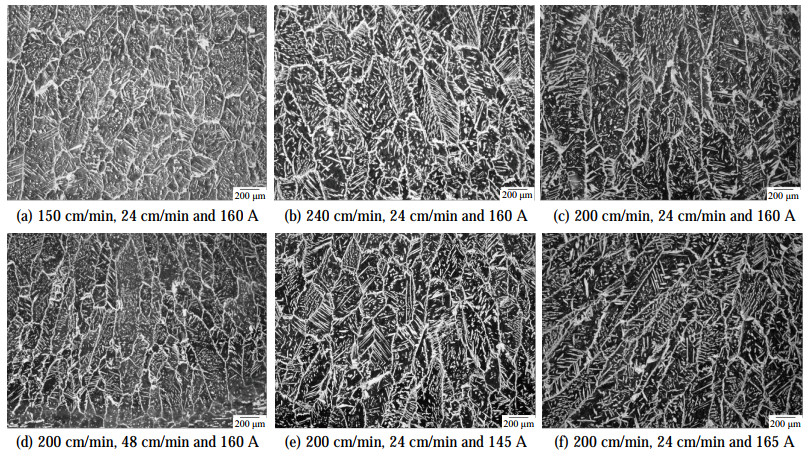Figure  7  Effect of WAAM process parameters on microstructure

Download: Full-Size Img

The WFS and welding current in Figures 7c and 7d are the same, but the welding speed is different at 24 and 48 cm/min, respectively. The microstructure in Figure 7c is mostly dendrite, and that in Figure 7d is mainly fine dendrite with minimal equiaxed structure. WS is an important influencing factor of arc heat input per unit time. When the WS is slow, the heat input of welding increases and the cooling speed of metal slows down, which is conducive to the formation of dendrites. On the contrary, the increase in WS accelerates the cooling speed, which is conducive to the formation of equiaxed crystals.

The WFS and WS in Figures 7e and 7f are the same, but the welding current is different at 145 and 165 A, respectively. The microstructure in Figure 7e shows the coexistence of equiaxed crystals and dendrites, and that in Figure 7f is dominated by dendrites with a small number of equiaxed crystals. The reason is that when the current increases, the molten pool temperature increases and the cooling speed slows down, which is conducive to the formation of dendrites.

In summary, WAAM process parameters affect the metal microstructure by influencing the cooling rate of the metal melt. The smaller the WFS, the faster the WS, which is beneficial to the generation of equiaxed crystals. The smaller the welding current, the faster the cooling speed of the metal melt, which is conducive to the formation of dendrites.

3.3   Response surface

3.3.1   Interaction of process parameters with weld bead width

The experimental design and experimental data obtained with the Design-Expert 8.0 software are shown in Table 2. In this study, 87 groups of experimental data were obtained to ensure the number of training samples in the later stages. In particular, 29 groups of experiments were carried out, and each group carried out three parallel experiments. The first 17 groups of data were used for response surface software fitting.

Figure 8 shows the bending degree of the response surface, that is, the level of interaction. From the bending degree of the surface in the middle part, we can conclude that significant interaction occurs between the weld bead width and the WS, welding current, and WFS. The reason is that when the WS increases, the heat diffusion of the weld bead per unit time slows down. However, when the welding current increases, the heat input also increases. As a result, the amount of melted wire per unit time increases, leading to changes in the weld bead width. No significant interaction is observed between the wire feed speed and welding current. The reason is that when the wire feed speed increases, the amount of wire filler per unit time also increases. An increase in the welding current means a high heat input. Therefore, when the WS is constant, no significant interaction exists between the weld bead width and the above two parameters.

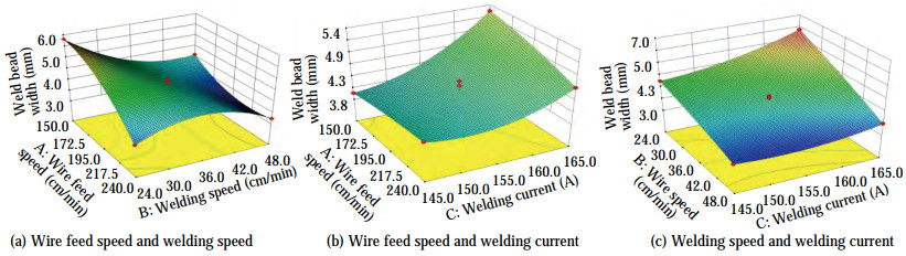Figure  8  Interactive effect of WAAM process parameters on weld bead width

Download: Full-Size Img

ANOVA of the response surface two-factor interaction model in Table 3 reveals that F=20.77, P=0.005, indicating that the model used in this experiment is significant. P_A, P_B, P_C, P_AB, and P_BC are all less than 0.05, indicating that the wire feed speed, WS, and welding current are three factors, and the WS has a significant influence on the interaction between the wire feed speed and welding current. The other interaction terms are less significant, which is consistent with the observation that the interaction between the wire feed speed and welding current is not significant in the 3D diagram. The model fit value R² = 0.935 3 is obtained, where R² is always between 0 and 100%. The higher the fit value, the better the model fits the data. The calculated R² indicates that the model has a good response value and good fitting of variation. The effect relationship of each factor is in the order of B (WS) > C (welding current) > A (wire feed speed). The influence of various factors on the weld bead width is not a simple linear relationship. According to the regression analysis of the experimental results and the establishment of regression models:

3.3.2   Interactive effect of process parameters on weld bead height

Figure 9 shows that the interaction between the wire feed speed and WS has a significant effect on the bead height. The reason is that when the wire feed speed increases and the welding current remains unchanged, the increase of WS results in less heat input to the filled wire and an increase in the bead height. No significant interaction is found between the bead height and the welding current, wire feed speed, welding current, and WS. The reason is that when the welding current and heat input increase, the amount of metal that can be melted increases. The increase in the wire feed speed also increases the amount of melt cover per unit time. With the increase in the WS, the bead height changes significantly.

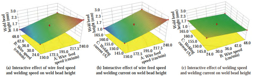Figure  9  Interactive effect of process parameters on weld bead height

Download: Full-Size Img

The principle of ANOVA in Table 4 is the same as that of the above analysis of the influencing factors of bead width. The model fit value R² = 0.949 8 is obtained, indicating that the model has a good response value and good fitting of variation. The effect relationship of each factor is in the order of A (wire feed speed) > B (WS) > C (welding current). The effect of the factors on the bead height is obtained through the regression analysis of the experimental results using the regression model:

In the above analysis, the maximum weld bead width was set as a numerical criterion for the comparison of experimental results. The obtained optimized process parameters are a wire feed speed of 200 cm/min, WS of 24 cm/min, and welding current of 160 A.

A single-layer weld bead formed under the above best process parameters is shown in Figure 10a. The surface of the weld bead is smooth without defects. As displayed in the cross-section of the weld bead in Figure 10b, the internal forming quality of the weld bead is good.

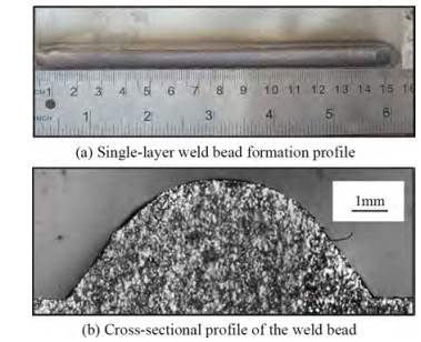Figure  10  Weld bead under optimized process parameters

Download: Full-Size Img

3.4   Validation of PSO-BP prediction results

In accordance with the topology and parameter setting of the BP neural network, the dimensionality of PSO was calculated as D = l* (m + n) + l + m. Population number N was set between 10 and 50, and N=40 was chosen for this work. The initial and termination weights were w_ini = 0.9 and w_end = 0.3, respectively. The total number of iterations was G = 100, and the learning factor c₁ = c₂ = 2. Figure 11 shows that the iterative convergence speed of the fitness values of PSO is faster and more stable than those of BP. In addition, PSO optimizes the BP connection weights while improving the overall performance of the network.

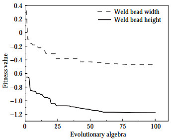Figure  11  PSO-BP bead width/height evolutionary process adaptation curve

Download: Full-Size Img

The distribution of PSO-BP predicted values, BP neural network predicted values, and actual output values is shown in Figure 12. A certain degree of coincidence is observed between the test sample data and BP-predicted values. Despite the error value between some groups of test samples and the predicted values in the middle of the graph, the results are still within the acceptable range.

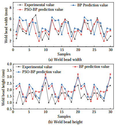Figure  12  Graph of predicted values and actual output values of PSO-BP and BP neural network

Download: Full-Size Img

The prediction errors of the PSO-BP prediction model in the figure are more stable and less floating than those of BP, indicating that the predictiveness of the BP neural network optimized by PSO is more stable, and the prediction accuracy is further improved.

Four groups of experimental data with different process parameters were selected and predicted, and the comparison results are shown in Table 5. The maximum absolute error of the prediction model of BP-PSO is 4.27%, and that of the BP neural network is 7.74%. Compared with the BP prediction model, the PSO-BP prediction model has a smaller error, and its predicted bead width and height are closer to the actual values.

4   Determination of the fitting function of the weld bead section

In the WAAM of metal parts, the dimensional accuracy and quality of the metal part are affected by the welding process, cross-sectional geometry of the single weld bead, and overlap of adjacent weld beads. Modeling and analysis of weld bead cross-sectional profiles provide the necessary morphological data for slicing, path planning, and process automation in WAAM.

For the visualization of the weld bead shape for dimensional prediction, the weld bead was first produced by a 3D scanner into an STL file, which was then processed by MATLAB image processing to calculate the average cross-sectional profile of the weld bead. The coordinates of the bottom two points and the top point of the cross-sectional profile were determined, as shown in Figure 13. The experimental data were then substituted into the coordinate points in turn, and their positions were idealized as symmetrical about the Y axis. The point coordinates were obtained from the weld bead cross-section size, and the parabola function model, cosine function model, and semicircle function model were selected. The weld bead cross-section fitting shape was obtained by MATLAB software fitting, as shown in Figure 14a. Finally, the mean square error of different models was calculated, and the fitting accuracy of different models was compared. Figure 14b shows the mean square error between different fitting functions and the actual weld bead coordinate points in the fitting process.

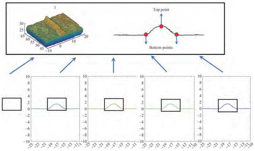Figure  13  Weld bead 3D scanner STL file with section coordinate points

Download: Full-Size Img

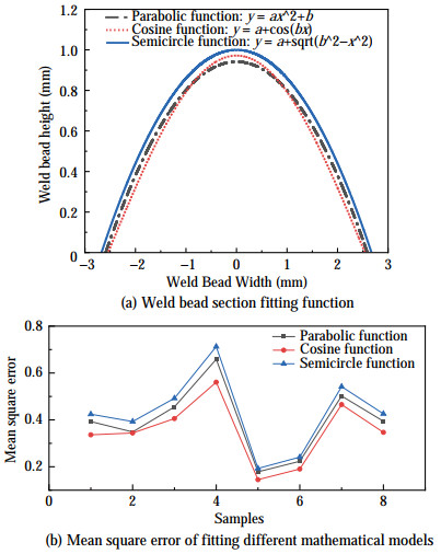Figure  14  Process of determining the optimal fit function for the weld bead cross-section

Download: Full-Size Img

Figure 14a shows the fitted shape of the weld bead cross-section. The coordinates of points were obtained from the weld bead cross-section size. Three function models, i.e., the parabolic function model, cosine function model, and semicircle function model, were selected to fit the shape of the weld bead cross-section. Another fitting was performed in MATLAB software. Figure 14b shows the mean square error of the different fitting functions related to the actual weld bead coordinate points during the fitting process. Here, the maximum fitting mean square errors of the parabolic function, cosine function, and semicircle function are 0.65, 0.46, and 0.71, respectively. The cosine function fitting is closest to the weld bead cross-section geometry, which serves as a guideline for multilayer multipass WAAM.

5   Conclusion

In this work, duplex stainless steel was formed through WAAM using tungsten inert gas. The effects of WAAM parameters and their interaction on forming dimensions were evaluated. The cross-sectional dimensions of the weld bead were successfully predicted using PSO-BP, which improved the prediction accuracy compared with that using BP. The fitting function of the single-pass single-layer weld bead section of duplex stainless steel WAAM was determined.

1) The weld bead width increases with the wire feed speed and welding current and decreases with the increase in the WS. The significant influence on the bead width is in the order of WS > welding current > wire feed speed. The weld bead height is positively correlated with wire feed speed but negatively correlated with the WS and welding current. The significant influence on the bead height is in the order of wire feed speed > WS > welding current.

2) The interactive effect between the wire feed speed and WS on the bead height is significant, but that between the welding current, wire feed speed, welding current, and WS is not significant. The interactive effect among the WS, welding current, WS, and wire feed speed on the bead width is significant. No significant interaction is found between the wire feed speed and welding current. The optimized process parameters for duplex stainless steel WAAM are wire feed speed of 200 cm/min, WS of 24 cm/min, and welding current of 160 A. WAAM process parameters affect the metal microstructure by influencing the cooling rate of the metal melt. The smaller the WFS, the faster the WS, which is beneficial to the generation of equiaxed crystals. The smaller the welding current, the faster the cooling speed of the metal melt, which is conducive to the formation of dendrites.

3) The maximum error of the BP neural network in predicting weld bead width and height is 7.74%. After PSO optimization, the maximum error between the predicted and experimental values of the BP neural network is 4.27%. With the fast convergence speed, the prediction accuracy is improved.

4) The maximum fitting mean square errors of the parabolic function, cosine function, and semicircle function models in the fitting function of the weld bead section are 0.65, 0.46, and 0.71, respectively, showing that the error of the cosine function model is the smallest and its fitting effect is the best.