1   Introduction

Turbulence parameterization is highly uncertain in both physical and sediment numerical models (Geyer and Ralston, 2015). In the past decades, the major focus on turbulence modelling is to suggest equations closures at various sophistication levels. Numerous modifications to these models have been proposed (Rodi, 1984; Chen and Beardsley, 1998; Umlauf et al., 2003; Burchard et al., 2014; Liu et al., 2022).

The k−kl turbulence closure scheme (Mellor and Yamada level-2.5, MY2.5, MY 1982) has been used widely in estuaries and coastal oceans. In the MY2.5, the vertical turbulent viscosity is calculated by solving the turbulence kinetic energy (TKE) equation and turbulence length scale equation. This scheme seems to work well for tidal-induced mixing in shallow waters (Chen and Beardsley, 1998), but further validation is needed for the estuarine regions. Several studies have been carried out to improve this turbulent model (Galperin et al., 1988; Burchard et al., 1998; Burchard and Bolding, 2001). A modification of the macroscale equation has been introduced, together with a new wall proximity function to investigate the vertical structure of open channel flows (Blumberg et al., 1992). Rodi (1984) significantly advanced the k−ε. Recent contributions paid particular attention to the buoyancy parameterization and model comparison (Burchard et al., 1998; Burchard and Bolding, 2001; Burchard et al., 2014). Umlauf et al. (2003) suggested a generalization of a class of differential length-scale equations typically used in second-order turbulence models for oceanic flows. Generally used models, such as the k−ε and the MY2.5, can be treated as special cases of this generic model. Recently, some studies have investigated physical and numerical turbulent-mixing behavior through numerical experiments (Reffray et al., 2015; Ralston et al., 2017; Costa et al., 2017; Tu et al., 2019; Choi et al., 2021).

Since vertical diffusion is one of the key processes for suspended sediment concentration (SSC) in estuaries, the uncertainty due to various turbulence parameterization schemes should be considered in the assessment of the reliability of the sediment transport model. Warner et al. (2005) evaluated the performance of four turbulence closure models and their influences on suspended sediment transport using a generic length scale method with several ideal cases based on ROMS. In this contribution, we carry out numerical experiments to investigate the impacts of turbulence parameterization on the suspended-sediment profile, together with different stability functions. We conducted the experiments by running FVCOM with various turbulence closure modules implemented in the General Ocean Turbulence Model (GOTM).

In recent years, since the reclamation on both sides of the waterway and the evolution of shoals, the deposition in local thalweg areas has aggravated to obstruct navigation (Lima et al., 2021; Wu et al., 2022). Yang and Wang (1994), and Chen et al. (2003) have conducted numerical simulations of the tidal wave and sediment transport in the Pearl River, but without systematic analyses in the Yamen Channel, which is one of the eight outfalls of the Pearl River. It is of great significance to investigate the hydrodynamics and suspended sediment transport in this area. Recently, some studies have been carried out in the Pearl River estuary (Zhang et al., 2019; Yang et al., 2022). To further investigate the turbulence simulation and better understand its impact on the sediment dynamics in the Pearl River Estuary, we conduct numerical simulations to investigate the sensitivity of turbulence parameterization on vertical distributions of velocity and SSC in the Yamen Channel. This paper is structured as follows: after describing the study area and observations (Section 2), we present three main modules of the numerical model together with model configuration (Section 3). Section 4 gives the sensitivity analysis of turbulence parameterization and model validation, followed by a detailed investigation of the spatial-temporal variations of SSC and intra-tidal variations of turbulent parameters, vertical velocity, and SSC. The conclusions are listed in Section 5.

2   Study area and observations

Yamen Channel, located at the head of the Huangmao Sea (HM Sea), is the westernmost one of the eight outfalls (YM: Yamen, HTM: Hutiaomen, JTM: Jitimen, MDM: Modaomen, HM: Hengmen, HQM: Hongqimen, JM: Jiaomen, HuM: Humen) of the Pearl River Delta (Figure 1). In Figure 1, Z2, Z3 and Z4 are sites for water levels. A3, A4, and A5 are for velocity and SSCs. The runoff of the Tanjiang River (TR) flows into HM Sea through the Yamen Channel. This typical tidal-dominated channel is an important navigable waterway, which is surrounded by extensive intertidal salt marshes and numerous tidal creeks. The annual discharge is about 196 × 10⁸ m³, which covers 6% of the total runoff of the Pearl River (Figure 1). Compared to the strong tidal current, the river flow appears weak. The average tidal range is approximately 1.24 m. The model domain is up to the Tanjiang River, and reaches the HM Sea downstream. A comparison between the Yamen and the Hutiaomen (HTM) at the HM Sea is shown in Table 1.

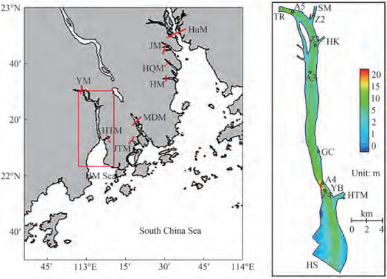Figure  1  The sketch and the local topography of the Yamen channel (the red rectangle, TR: Tanjiang River, HS: HuShan, YB: Yamen Bridge, GC: GuanChong, HK: Hukeng, SM: Sanjiang Mouth.)

Download: Full-Size Img

The medium diameter of the suspended load is less than 0.1 mm and the diameter of sediment particles from the upstream during ebb tide is larger than that from the outer sea during flood tide. In flood season, flow with high SSC enters the Yamen channel. The mean grain size is about 5 μm. The sediment is mainly transported in suspension. The particle diameter of bed sediment between 0.005-0.05 mm covers about 50%, and the median particle size is less than 0.05 mm.

3   Numerical Model

3.1   Hydrodynamic model

We adopted an unstructured-grid, three-dimensional primitive equation community ocean model FVCOM (Finite Volume Community Ocean Model) in this study (Chen et al., 2007). It solves the governing equations in unstructured triangular mesh by finite-volume method, which provides accurate conservations of mass, momentum, heat, and salt. This model has been applied to a number of estuaries and coastal oceans characterized by highly irregular geometry, large intertidal salt marshes, and steeply sloping bottom topography (Ding et al., 2013; Lai et al., 2015; Sun et al., 2016).

3.2   Suspended sediment model

Suspended sediment is simulated by the three-dimensional suspended sediment equation in σ-coordinate:

where A_h is the horizontal diffusion coefficient, K_h is the vertical diffusion coefficient, C is the suspended sediment concentration, ω_s is the settling velocity, H is total water depth, and (u, v, w) represent horizontal and vertical velocity, respectively.

Sediment particles near the bed can be re-suspended when the bottom bed stress exceeds critical stress. The bottom boundary condition is determined by near-bed sediment flux (van Rijn, 2005; Li et al., 2008):

where F_s is near-bed sediment flux, E is erosion flux, and D is deposition flux. The deposition rate (D in kg/(m²s)) is determined as the mass that is removed from the suspended load and integrated into the bed. It depends on the particle's sinking velocity ω_s, and the near bottom concentration C_b in kg/m³:

Erosion is an instantaneous process that is initiated when the bed shear stress exceeds a critical value τ_ce, which is derived from the critical Shields parameter (Warner et al., 2008).

where Q is the erosion flux, P_b is the bottom porosity, F_b is the fraction of sediment and τ_ce represents critical shear stress.

In terms of the initial conditions, the suspended sediment concentration is zero for the normal component on the fixed boundary. At the outflow open boundary, it is determined as $ \frac{\partial C}{\partial t}+v_n \frac{\partial C}{\partial n}=0$, vn is the normal velocity component, and n is the normal direction to the open boundary. For the inflow, C = C₀, where C₀ is the given values.

The sediment bed is represented by 3-D arrays with a user-specified, constant number of layers beneath each horizontal model cell. At the beginning of each time step, active-layer thickness z_a is calculated based on the relation (Warner et al., 2005, W2005)

where τ_b is bottom stress, τ_ce is the critical stress for erosion, D₅₀ is the median particle size, and k₁ and k₂ are empirical coefficients (0.007 and 6.0, respectively). The thickness of the top bed layer has a minimum thickness equivalent to z_a.

3.3   Turbulent closure

The Reynolds stress tensor and the turbulent tracer flux need to be parameterized to close the hydrostatic primitive equations that resulted from the Reynolds-averaging Navier-Stokes equations. The transport equations are parameterized by approximations of the third-order moments and pressure correlation terms. Additional scaling and boundary layer assumptions further reduce the set of equations of the Reynolds stresses and turbulent scalar fluxes in the form as follows:

with

where ρ is total density, and U and V are velocity of the mean components in the horizontal directions, respectively. u', v', and w' are the turbulent components of velocity in the horizontal and vertical directions, respectively. K_M is the turbulent viscosity, K_H is the turbulent diffusivity, and S_M and S_H are stability functions that describe the effects of shear and stratification, respectively. υ and υ_θ represent molecular viscosity and diffusivity, respectively. l is turbulent length scale.

The GOTM developed by Umlauf and Burchard (2003)is a community turbulence module and is continuously upgraded (Burchard et al., 2008; Reissmann et al., 2009; Umlauf and Burchard, 2011). This module includes two typical turbulence closure models, (1) k−kl equation and (2) k−ε equation. Both turbulence module groups include the original code with a Richardson number cut off between 0.2 and 1.0. The GOTM has been coupled to FVCOM through an interface library, thus one can select different turbulence schemes to replace the default setup of the MY2.5 turbulence closure scheme.

The turbulent closure schemes rely on the stability functions parameterizing the pressure-strain correlation terms of the Reynolds stress (Burchard and Bolding, 2001). Each stability function considers a different approximate equilibrium of the five pressure-strain effects, including isotropy, shear production, buoyancy production, non-isotropic contribution and vorticity contribution. Five different stability functions have been explored: the modified MY2.5 which only contains isotropy and shear productions (Galperin et al., 1988), KC (Kantha and Clayson, 1994) which includes both isotropic and non-isotropic contributions; BB which contains the isotropy shear and buoyancy turbulence productions (Burchard and Baumert, 1995); CA (Canuto et al, 2001) which includes all five pressure-strain terms; and CB (Burchard and Baumert, 1995; Canuto et al., 2001) which was deduced for an equilibrium state that turbulence dissipation balances turbulence productions. We implemented the original MY2.5, modified MY2.5 (G1988), and the KC stability functions in the k−kl equation and the other three stability functions (BB, CA, and CB) for the k−ε equation model (Table 2).

3.4   Model configuration

The model area is discretized by non-overlapping triangular cells with a horizontal resolution of 20-80 m. Twenty even sigma layers are separated in the vertical direction, which allows for a slightly smooth representation of finite-amplitude irregular bottom bathymetry. The total numbers of triangular elements and nodes are 6 295 and 3 563, respectively. The time step for the external mode is 0.1 s.

The model is forced by river flow at the upstream riverine boundary and by water level at the southern open boundary. Tanjiang River, Sanjiang Mouth, HuKeng, and HTM channel are all input sources of riverine discharges and SSCs. Hushan is the downstream control boundary with water level extracted from the tidal dataset TPXO7.2 (Egbert and Erofeeva, 2002). Topography is based on the nautical maps published Dec. 2004 as the model terrain(Figure 1).

The wind is weak during the simulation period, thus wind-induced wave effects and wind forcing are not included in these simulations. We chose the Smagorinsky turbulence parameterization method for the horizontal diffusion coefficient.

Since the SSCs are relatively small (0.02-0.4 kg/m³) along the channel, and the influence of turbid water on particle settling is neglected, the settling velocity is set as a constant of 0.75 mm/s for simplicity. The critical erosion shear stress is set to 0.04~0.06 N/m², and a mean value of 0.05 N/m² is used in the simulations. The erosion constant is 5×10⁻⁵ kg/(m² s) (Table 3).

4   Results and analysis

4.1   The sensitivity analysis of turbulence closures

We conducted sensitivity analysis based on turbulent closure methods using the k − ε equations with stability functions of CA, CB, and BB, k − kl with KC, MY2.5, and G1988, and Analysis (ANA). The ANA is an algebraic expression for the turbulent viscosity asK_M = ku_* z (1 − z/H), where k is a coefficient, u_*, frictional velocity, z, distance above the sea bed, and H, total water depth. Z4 is located near the Yamen Bridge with a depth of ~10 m. We chose this site to investigate the influence of turbulence closure schemes on the vertical distributions of velocity and SSC.

4.1.1   Vertical profile of turbulent variables

As a measure of turbulence intensity, TKE is one of the most important variables related to the momentum transport through the bottom boundary layer (BBL). Figure 2a shows that the k − kl with the three stability functions of KC, MY2.5, and G1988 generates almost identical patterns. The k − ε produces a notable difference among the three different stability functions, especially in the lower half of water depth. The values of CB and BB are ~2 times larger than that of CA. ANA would become more turbulent than the other methods.

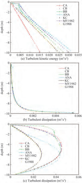Figure  2  Vertical distribution of turbulent parameters

Download: Full-Size Img

Turbulent dissipations computed by different stability functions keep in good consistency, except that ANA would dissipate strongly near the BBL (Figure 2b). Generally, ANA would overestimate both TKE and turbulent dissipation especially near the BBL.

The k − kl generally underestimates turbulent viscosity by ~40% compared to that of k − ε and ANA (Figure 2c). The maximum values of k − ε and ANA are almost identical. The profile of turbulent viscosity demonstrates asymmetrical characteristics for all turbulent schemes. However, ANA and k − kl show an asymmetry biased towards the lower layer of water depth, whereas k − ε simulates an asymmetry towards the upper layer.

4.1.2   Vertical profiles of velocity and SSC

The vertical velocity profile shows two typical different patterns, especially in the surface layer (Figure 3a). The k − kl with the three different stability functions and ANA produce anomalously high surface currents. This behavior has been documented (Blumberg et al., 1992; Burchard et al., 1998; Burchard and Bolding, 2001; Warner et al., 2005). Simulations by Warner et al. (2005) in open channel show that the original MY2.5 and k − kl with parabolic wall function have abnormally high surface currents. This is consistent with the results of other turbulence schemes, including k − ε, k −ω, ANA, and k − kl with improved open channel wall function (Warner et al., 2005). In this paper, k − ε schemes (CB, CA, BB) produce results that agree closely, while the surface flow velocities obtained using the k − kl schemes including G1988, original MY2.5, KC, and ANA are excessively large. Warner et al. (2005) pointed out that the wrong wall function produces an incorrect mixing length scale, which leads to the underestimation of turbulent visibility far from the boundary. Moreover, other important consequences, besides the resultant higher depth-averaged velocities in the open channel, would also exist in the estuary. For instance, the mixing of fresh water and saline water in the estuary has a critical impact on the estuarine gravitational circulation (Hansen and Rattray, 1965). The gravitational circulation is suppressed when the vertical mixing is strong, and vice versa. Moreover, when surface velocity in the estuary is enhanced artificially, more water flux flows seaward in the upper layer. Due to the continuity, additional seawater should enter the estuary in the lower layer. This process will not only falsely enhance the estuarine circulation, but also affect the exchange capacity and time scale of material transport. In W2005, two wall functions, i. e., the parabolic wall function and the open channel wall function, were introduced into the k − kl scheme. The results show that the former made no improvement, but the open channel function eliminated the abnormally high surface current and produced results similar to those by k − ε, k − ω, etc. (Warner et al., 2005). In this paper, we implemented three stable functions in the k − kl and k − ε. The results show that an abnormally high surface current remains without introducing the correct wall function regardless of the stability functions.

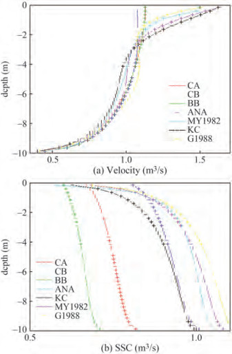Figure  3  Vertical distribution of vertical velocity and SSC

Download: Full-Size Img

Different stability functions impose distinct influences on the vertical distribution of SSCs (Figure 3b). The k − ε appears less gradient in the vertical direction than k − kl near the upper layer (0-5 m). Suspended sediment distributes more uniformly in the vertical due to a larger diffusivity coefficient and an asymmetry towards the upper layer. Simulations by k − ε may lead to wide variations in the magnitude of vertical-averaged SSCs. In W2005, ANA and k − ω generated the largest SSC. The k − kl with parabolic wall function and the original MY2.5 produce the lowest values. The k − ε and k − kl with open channel wall functions are in between. Nevertheless, their vertical distributions of SSC display extremely similar patterns. In our simulations for the Yamen Channel, SSC based on ANA and k − kl schemes are relatively large. Results by KC and CB are very close except obvious decrease by KC due to the small turbulent diffusion in the surface layer. The results by CA and BB are smaller. This might be attributed to the relatively large turbulent viscosities of the CA and BB, which weakens the estuarine circulation and reduces upstream sediment transport.

Generally, the k − kl closure scheme depends on wall function, which should be chosen with caution. Several alternate wall functions are proposed to produce an apparently correct parabolic turbulent viscosity profile. Given certain boundary and initial conditions, k − ε produces more intensive vertical mixing than k − kl. On the other hand, the k − kl tends to generate stratification. According to the vertical profile of turbulent parameters, vertical velocity, and SSCs, the CB function based on k − ε generates reasonable patterns. Thus, we apply this parameterization to the model validation and further analysis in the Yamen Channel.

4.2   Model validation in the Yamen Channel

Based on the above sensitivity analysis, the k − ε with CB stability function is chosen to validate the simulated results. Three metrics are used to quantify the agreements between observed and modeled data of water level, velocity, and SSC. A skill that has been widely used is written as (Willmott, 1981; Li et al., 2005):

where the subscript'o' and 'm' indicate observed and modeled data respectively, and'n' is the number of total time series. Another index to evaluate the absolute deviation of velocity and suspended sediment is mean absolute error (MAE):

The deviation of the current direction is computed using mean absolute error coefficient (MAEC) defined in equa‐ tion (10). Compared to equation (9), equation (10) empha‐ sizes the contributions in the main directions and weakens the influences that arise from the slow slack flow which might be measured less precisely. The weights are chosen as square velocity amplitudes in the sense of kinetic energy.

where u is the velocity, and others are the same as the above.

We validated the modeled results against the observa‐ tions during April 11-12 in 2005 (Figure 4). Though the discrepancy increases slightly toward the downstream, the predictions show good agreement with the observations. We collected the statistics of water elevation with two metrics, MAE and Skill (Table 4). Skills are 0.99, and MAEs are less than 0.08 m at the three stations.

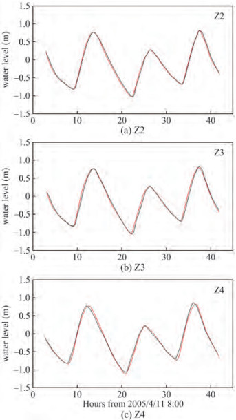Figure  4  Validation of water elevation (black line for the modeled, red line for the observed)

Download: Full-Size Img

The comparisons between the modeled and observed velocities at the three stations are shown in Table 5. MAEs of the velocity are 0.03-0.09 m/s. As the modeled and observed data are not at the exactly same location, and combined with grid resolution, some large deviations emerge. However, the Skills show good performance. MAECs of current direction are less than 11°, and Skills are larger than 0.9.

The comparisons of SSCs between the measured and predicted are shown in Figure 6 during the spring tide. Circle ("○") represents the measured and the thin line ("—") is the computed. The SSCs are lower than 0.4 kg/m³; in contrast, MAEs are less than 0.07 kg/m³. We concluded that the trend of SSC is considerably identical. According to the comparisons, the simulations are acceptable.

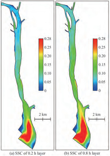Figure  6  SSC during flood maximum (kg/m³)

Download: Full-Size Img

4.3   Spatial variations of SSC

The SSC fields of 0.2 h and 0.8 h layers during the flood and ebb tide are presented in Figures 6 and 7, respectively. The SSCs to the south of Yamen Bridge are higher than that to the north during the flood tide, which vary from 0.1 to 0.3 kg/m³ and are basically lower than 0.1 kg/m³ to the north of the YB.

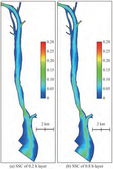Figure  7  SSC during the ebb maximum (kg /m³)

Download: Full-Size Img

The SSCs of each layer during the flood tide are higher than that during the ebb tide, which can be attributed to the tidal asymmetry in the HM Sea. The mean duration of the ebb tide is longer than that of the flood tide, and tidal currents adversely. In the dry season, the duration of the ebb tide is longer than that of the flood tide for 1-2 hours. The bidirectional current flows mainly along the deep channel. Due to the tidal asymmetry in the channel, the flow velocity is smaller during the ebb tide than during the flood tide. Therefore, suspended particles tend to settle and deposit to the bed, and fewer sediment particles on the bed can be re-suspended correspondingly.

The SSCs near the estuarine bar from the HTM to the middle channel are relatively high. At the same station, SSCs during the flood tide are higher than that during the ebb tide. The SSCs vary from 0.03 kg/m³ to 0.14 kg/m³ in the HM Sea. Due to the complicated interactions between the freshwater and shelf saline water and the effect of local terrain, the SSCs exhibit obvious variations in the vertical.

4.4   Intratidal variations

According to the above analysis, we chose the results based on k − ε and CB stability function to investigate the temporal variations of turbulent viscosity, turbulent kinetic energy, dissipation, velocity and SSC at site A3, which is located near the thalweg of the upstream channel in the Yamen Channel. The tidal currents exhibit a typical flood-dominated asymmetry. At high and low water, the velocity is extremely weak (Figure 8a). Flood current is larger than the ebb current of ~0.2 m/s, which is referred to the tidal velocity asymmetry (Song et al., 2011; Gong et al., 2016). The turbulent viscosity is extremely small at both high and low tide levels due to slack water. On the contrary, it is much greater at the maximum ebb and flood tide, which shows a positive correlation between turbulent viscosity and tidal velocity. The turbulent kinetic energy also shows similar variations. However, there is no obvious trend of dissipation. In W2005, the dissipations based on different schemes are nearly identical except MY2.5. Contrastingly, the results of turbulent kinetic energy are different. Moreover, the comparisons in W2005 are only at a timing of maximum ebb. Nonetheless, the simulated SSCs are considerably consistent except for that by MY2.5. This issue deserves further investigation: why does the abnormally high surface velocity have almost no impact on SSC?

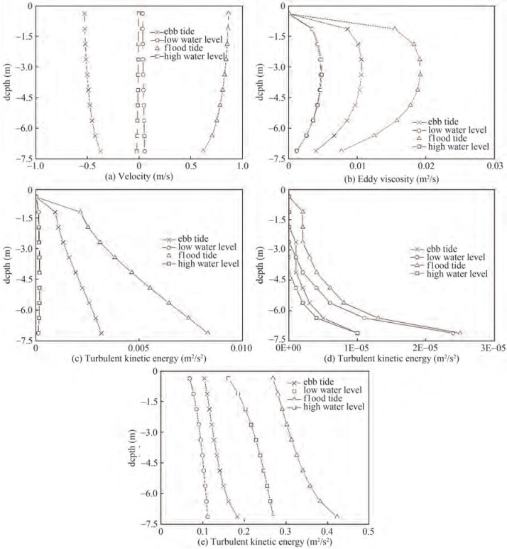Figure  8  The vertical distribution of the simulated results during a tidal cycle at the A3

Download: Full-Size Img

In Figure 8d, the dissipations scarcely change corresponding to the tidal velocity similar to turbulent kinetic energy and turbulent viscosity. At high water levels, the dissipation is the smallest, while the largest value is at maximum flood tide. The turbulent dissipation at maximum ebb tide and low water level fall in between. We speculate that this temporal variation is due to the local instantaneous water depth, which may restrict the development of turbulence, and ultimately determine the turbulent dissipation $ \left(\frac{k^{1 / 2}}{l}\right)$ together with the tidal velocity. At high water levels, due to small velocity and large water depth, the turbulent dissipation is significantly weak. At maximum flood tide, the flow velocity is large, and the water level is close to the mean tide level; therefore, the turbulent dissipation maintains large.

Due to the re-suspension and increased sediment-carrying capacity, SSC is the largest at maximum flood tide. At high water levels, in pace with the decrease of velocity, the sediment gradually settles and the SSC decreases. Settling/ scour lag is an interesting issue calling for special attention. As an agent, the sediment response time can be expected to be approximately equal to the vertical distance which scales the fall off sediment concentration divided by the suspended sediment fall velocity (Friedrichs et al., 1998). Analogously, the sediment response time is about 20 min in the Yamen Channel. Therefore, it can be prudently considered that the lag effect is not significant. After the high water levels, the sediment keeps settling. The maximum ebb velocity is generally less than 0.5 ms⁻¹, which is not strong enough for sediment incipience corresponding to a median particle size of 0.05 mm. Therefore, during the whole ebb period, the SSC would not increase. This process can also be seen in Figure 5, where the period of SSC is about semi-diurnal rather than quarter-diurnal. Although the turbulent viscosity is the greatest at maximum flood tide (Figure 8d), a certain vertical gradient of SSC still exists due to the resuspension from the seabed acting as a sediment source. At high water levels, the vertical distribution of SSC is more uniform than that at maximum flood tide. Since the weakened turbulent mixing and the sediment settling result in more suspended sediment loss in the upper layer than in the lower layer, the SSC in the surface layer is slightly smaller consequently. At maximum ebb tide, although the suspended sediment cannot be supplemented by the resuspension, the SSC is uniform in the vertical due to the enhanced turbulent mixing. At the low water level, the SSC is extremely low, and the vertical variation is insignificant.

Figure  5  Comparisons of SSCs during the spring tide

Download: Full-Size Img

5   Conclusions

Based on the coupled Sed-FVCOM system with two kinds of turbulence closure schemes with different stability functions implemented in the General Ocean Turbulence Model (GOTM), we carried out numerical experiments to examine the effects of turbulence parameterization on the temporal and spatial distribution of suspended sediment in a natural tidal channel.

The k−kl scheme with three typical stability functions produces anomalously high surface currents. It can be attributed to the improper wall functions embedded in the original MY2.5 closure scheme, which produces an incorrect length scale and underestimation of the turbulent viscosity near the surface. One should use the original MY2.5 with caution and select the proper wall function. The effects of each stability function on vertical dissipation are extremely small. By contrast, the k−kl and k−ε can produce significantly different turbulent viscosity in the vertical, and thus turbulent diffusivity. We concluded that under specified boundary and initial conditions, k−ε turbulence schemes generally produce more intensive vertical mixing than the k−kl does.

Allowing for the simultaneous depositional process during erosion near the water-sediment interface, we applied k−ε with CB stability function in the Yamen channel, one of the eight outfalls of the Pearl River. During a tidal period, the turbulent dissipation show highly similar trends while the patterns of the SSCs differ significantly. Although velocity, turbulent viscosity, and TKE keep similar trends and magnitudes respectively, the SSCs show different patterns between low and high water due to complex mechanisms.

This paper illuminates the influence of two kinds of turbulent closure schemes with several different wall functions on velocity and SSCs in the Yamen channel, which is important to the Guangdong-Hong Kong-Marco Greater Bay Area. Our findings provide insights into, and references for, turbulent and sediment parameterization for researchers and estuarine management.