1   Introduction

Bigger ships require bigger propellers to move them and the flow velocity in the vicinity of these propellers is very high. The high flow velocity reduces the pressure on the propeller blades leading to the formation of cavitation. Due to this reason, cavitation is a very hard-to-avoid incident, especially for large commercial ships. Cavitation is an unwanted phenomenon because it leads to erosion (Koksal et al., 2021) and noise (Tani et al., 2019). It also decreases the hydrodynamic efficiency of the propulsion system (Ebrahimi et al., 2021). Research on marine propeller cavitation has increased substantially in recent years. Some are briefly noted in this study.

Many attempts have been made to decrease cavitation size by configuring the propeller geometry. The installment of vortex generators on the hull was one of the recent attempts that resulted in milder cavitation (Huang et al., 2020). Leading-edge tubercles on the sheet cavitation development of the propeller were investigated by (Stark et al., 2021). It was concluded that these tubercles reduced sheet cavitation for heavily cavitating propellers. An improvement of 6.5% was achieved in propulsive efficiency. Some others tried increasing the skewness of the propeller blades. These studies generally show that larger propeller skew leads to smaller cavities. For instance, Feng et al. (2019) conducted numerical investigations on the DTMB 4119 propeller having balanced and biased skew to see the effect of the cavitation on pressure-induced fluctuations. The study revealed that at the same operating condition, the vapor volume is smaller for balanced skew than the biased skew marine propeller. Additionally, it was shown that the propeller skew type has little effect on pressure fluctuations and the balanced propeller had slightly lower pressure fluctuations than the biased propeller. The influence of propeller skew on tip vortex cavitation (TVC) was studied using the Large Eddy Simulation (LES) using one blade (Hu et al., 2021). Calculations were conducted at two different advance ratios with constant propeller revolution. Different blade geometries were used by varying the radial skew distribution while other parameters were kept constant. The authors concluded that increasing the skew reduces the tip vortex cavity intensities gradually and the length of the sheet cavitation bubbles also decreases in the chordwise direction.

One of the most difficult topics in this field is to capture the TVC, which has notable effects on ship propulsion. Many recent studies focus on this specific type of cavitation. A recent numerical and experimental investigation on propeller TVC was conducted by (Yilmaz et al., 2020a). The measurements of the open water performances and tip vortex inception were carried out in the Shanghai Jiao Tong University cavitation tunnel. The authors have implemented an approach of meshing, which they call Mesh Adaption Refinement for cavitation Simulations (MARCS), to capture the tip vortex in a propeller slipstream. This approach consists to create an adaptive mesh in the region where the TVC can occur. Results showed that good accordance with experiments was noted for propeller hydrodynamic performance, cavitation formation, and tip vortex inception.

Modeling of the TVC is significantly harder for propellers behind the hull. A study of propeller-hull-rudder interaction using computational and experimental fluid dynamics approaches was conducted by (Yilmaz et al., 2020b) under cavitating conditions. MARCS, which showed good performance in open-water conditions, was less satisfactory in behind-the-hull conditions. Another study of similar focus was conducted by (Ge et al., 2020). They predicted the cavitation of a marine propeller operating behind a hull of a model container vessel by RANSE-based CFD simulations. The study revealed that with tip-refined mesh, they were able to resolve cavitation and bursting. Long et al. (2019) numerically solved the cavitating turbulent flow around a propeller behind the hull. They have obtained good agreement with measurements in terms of propeller hydrodynamic performance and cavitation pattern.

In this study, we utilized a commercial computational fluid dynamics code to resolve the cavitating flow around a marine propeller in open water. In the next section, we present the non-dimensional parameters governing the hydrodynamic performance of a cavitating marine propeller. We, then, introduce the propeller geometry and the simulation test matrix in Section 3. The equations related to hydrodynamic propeller performance and the mathematical background of CFD simulations are given in Section 4. In Section 5, we explain the numerical implementation and the grid sensitivity analysis. Results are presented in Section 6 in two subsections. CFD simulations of open-water tests under different cavitating conditions are given in the first subsection, while the second subsection is devoted to the propeller's behavior in behind-the-hull conditions. The paper is finalized with concluding remarks in Section 7.

2   Non-dimensional parameters of a cavitating marine propeller

There are three necessary conditions for a model and a full-scale sized structure to be considered as "similar", i.e., geometrical, kinematic and dynamic.

Similarities. For two structures to be geometrically similar, they should have the same shape at different scales. Kinematic similitude for a propeller can be achieved at the same advance ratio. Dynamic similitude requires the ratio of forces between the model and the full scales to be constant. Inertial, viscous and gravitational force ratios between the model and the full-scale structure should be constant.

For propellers, geometrical similarity is similar to ships. Both propellers should have similar shapes and all propeller dimensions should have the same scale ratio. Kinematic similarity requires that velocities at any corresponding points of the two propellers must be proportional by a constant scale factor. This can be satisfied by setting the advance ratio equal for both propellers. However, satisfying the dynamic similarity is more complex than the other two.

The hydrodynamic performance of a propeller is under the effect of several non-dimensional parameters. These are the Reynolds number, the Froude number, the Cauchy number, the Mach number, the Weber number, the Euler number, the Helmholtz number and the Strouhal number. These parameters are crucial to satisfy the dynamic similarity problem for a cavitating marine propeller. However, this is a very hard task with so many numbers involved in the process and one has to make some assumptions to simplify the problem. The Specialist Committee on Hydrodynamic Noise on the 28^th ITTC (2017) states that "not all similitude requirements can be met with a single scale model". In this respect, observation of the flow physics around the propeller will allow us to make proper assumptions about its hydrodynamics. In this respect, we assume that viscous forces, gravitational forces, forces due to elastic compression and the free surface effects have minimal role in propeller hydrodynamics. We define the hydrodynamic performance of a propeller by the forces and moments acting on it. Considering the above-mentioned assumptions on the thrust and torque coefficients of a propeller and after following a proper non-dimensionalization process, we will find that they are functions of the Euler and Strouhal numbers. However, the Euler and Strouhal numbers have different naming in propeller hydrodynamics: we use cavitation number instead of the Euler number and advance ratio instead of the Strouhal number. In mathematical terms, we define the thrust and torque coefficients as a function of these two numbers:

The hydrodynamic performance of a marine propeller depends on the cavitation number σ and the advance ratio J. When the propeller performance is known with respect to changes in these variables, it is also possible to graph the cavitation bucket diagram as is given in (Alimirzadeh et al., 2016). In this study, we will consider these two non-dimensional variables to understand the behavior of E779A propeller in open-water and behind-the-hull conditions.

3   The propeller geometry

INSEAN E799A is a four bladed, fixed pitch, low skew and right-handed propeller designed in 1959 by the Italian ship model basin. The propeller is one of the widely used benchmark cases for experimental and numerical investigations. The geometrical description and main particulars of the propeller model are given in Figure 1 and Table 1.

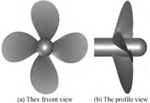Figure  1  Geometry of the INSEAN E779A propeller

Download: Full-Size Img

4   The mathematical background

The details of the numerical procedure used are shown. There are two different cases in this study; open-water performances prediction in cavitating and non-cavitating cases. The hydrodynamic propeller performance is estimated for both cases. This section first briefly explains the open-water propeller parameters and then continues to present the mathematical background of RANSE-based CFD simulations.

4.1   Open-water propeller performance equations

As previously shown by proper non-dimensionalization, the hydrodynamic performance of the propeller relies on the advance coefficient and the cavitation number. There are various forms of the cavitation number but in this study, we will be considering the formation of cavitation on marine propellers. Therefore, it is suitable to use the rotation rate of the propeller instead of the fluid velocity. In this respect, the cavitation number is calculated by

Here, p_v is the vapor pressure, n is the propeller revolution and D is its diameter. The open-water propeller performance of the propeller is defined by the following non-dimensional parameters:

These parameters are given with respect to the advance coefficient J. It is given by:

If the propeller is non-cavitating, we can define the hydrodynamic performance of the propeller with respect to J only, given in equation (6). If it is a cavitating propeller; then, we will also require the cavitation number given in equation (2) to assess K_T and K_Q generated by the propeller.

4.2   Non-cavitating case

For the non-cavitating case, the fluid medium consists only of water. The conservation form of the unsteady Navier-Stokes equations for single fluid has been numerically solved. The equations are defined as follows:

Here, u_i denotes the velocity components, P is the pressure on the fluid particle, ρ is the water density, μ is the dynamic viscosity and ρu'_i u'_jterm expresses the Reynolds stresses.

4.3   Cavitating case

For the cavitating case, the computational domain consists of a single fluid represented by a homogeneous mixture of two phases (water and vapor). The continuity and the momentum equations of the mixture flow are defined by

The mixture density and the viscosity are expressed as

where α is the vapor volume fraction and m, v, and l denote mixture, vapor and liquid phases, respectively. An additional transport equation is solved for α to close the equations. The cavitation model used in this study is developed by Schnerr and Sauer (2001). This model was found to yield the most accurate cavitation and thrust prediction for a marine propeller (Lee et al., 2021). Along with the continuity equation (9), it solves the vapor volume fraction with the following transport equation:

The source terms R_e and R_c account for the mass transfer between the vapor and liquid phases in cavitation. These source terms were derived from the bubble dynamics equation of the generalized Rayleigh-Plesset equation and they are written as follows:

The bubble radius R_B is calculated by

where n_b is the bubble number density. A default value of n_b = 10¹³ is used here. The source terms R_e and R _c in the transport equation approach to zero when α = 0 and α = 1.

5   Numerical implementation and grid sensitivity

The computational domain is divided into two cylindrical regions. The first is the rotational block surrounding the propeller. The second region is the stationary block that covers the rotational region. The inlet and outlet are situated at 1.5D and 3.5D from the propeller disc respectively (Watanabe et al., 2003). The curved surface of the stationary region is located at 1.4D. Poly-hexcore (mosaic) grid type in Ansys Fluent Meshing is used to build the mesh in this study. Two refinement zones are identified, namely Zone 1 and Zone 2 to catch the tip and the hub vortex. The cylindrical shell of Zone 1 that extends to the propeller disc was removed in Figure 2(a) for better representation of the computational domain. Three different grids are tested to understand the effect of the grid on results, the grid sensitivity is studied by using a grid refinement ratio $ r_G=\sqrt{2}$(Stern et al., 1999). Some views of the grids are given in Figure 2(b). For the fine mesh, ten layers are attached to the blade surfaces. The first cell height off the solid surface for the fine mesh is approximately 0.00132D. Wall y+ range is within 2-81. The details of the grid system for sensitivity analysis are given in Table 2.

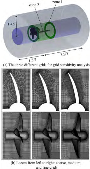Figure  2  The details of the computational domain

Download: Full-Size Img

The Navier Stokes equations are solved using the commercial code Ansys Fluent V. 21 based on finite volume method. The turbulent flow in this study is modelled using the k-ω SST model (Sezen et al., 2021). The water flow is considered as steady state and incompressible. Pressure-based solver is used. The Green-Gauss-Cell-based approach and the SIMPLE algorithm are selected for the pressure-velocity coupling which is known for its robustness. PRESTO method is utilized as the interpolation scheme for calculating cell-face pressure, which is frequently used for flows involving steep pressure gradients or in strongly curved domains. The second-order upwind method is used for Pressure, Momentum, Turbulent Kinetic Energy and Specific Dissipation Rate. The moving reference frame (MRF) method is used implemented to represent the propeller's rotation.

6   Results

Results are presented in two subsections. The first subsection is devoted to results obtained from CFD simulations of open-water propeller tests in cavitating and non-cavitating cases. The second subsection presents calculation results for behind-the-hull condition. The open-water results from the first subsection is given as input to the second subsection.

6.1   Open-water propeller test results

The open-water performance of the non-cavitating propeller is handled to validate the numerical approach. Therefore, in this section, the propeller hydrodynamic performance is only a function of the advance coefficient J. The experiments of the open water propeller were performed at the INSEAN medium-size longitudinal towing tank (Salvatore et al., 2006). The comparison of results is given in Figure 3.

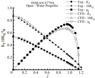Figure  3  Open-water propeller performance of INSEAN E779A propeller compared with experiments

Download: Full-Size Img

Thrust and torque coefficients are calculated at the advance ratio of J = 0.747 and compared with the experimental data. Results are summarized in Table 3, the error percentages with the fine grid are found to be the lowest in open-water propeller performance. Slight differences in the thrust and torque values at low advance ratios are observed as compared with the experiments. The discrepancy on the open-water propeller efficiency at high advance ratios are visible in the results but the overall agreement is found to be satisfactory.

Figure 4 shows the cavitation pattern at the advance ratio J = 0.83 and the cavitation number σ = 1.763. We did not only examine the quantitative data but also qualitative data from CFD in understanding the grid sensitivity. In this respect, the tip vortex was visualized with these grids (Sezen and Atlar, 2022). It was not possible to capture the cavitation pattern with the coarse and medium meshes. However, the fine mesh was partially able to capture the tip and hub vortex.

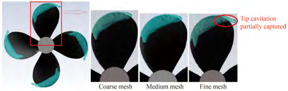Figure  4  The cavitation pattern with different grids at J = 0.83 and σ = 1.763

Download: Full-Size Img

Cavitation patterns at different advance coefficients and cavitation numbers are given in (Vaz et al., 2015). Here, we make a comparison of the obtained cavitation in our simulations using the published results in the reference paper. Results of different computational models submitted by seven organizations including our numerical results are shown in Figure 5. As it can be seen from the results of our study, we partially managed to capture the tip vortex. The hydrodynamic performance of the propeller at same advance coefficient of J = 0.71 with different cavitation numbers are given in Figure 6(a). Here, we see that the hydrodynamic efficiency is decreasing with decreasing cavitation number. This means that at J = 0.7, the propeller performance declines with increasing cavitation size. The cavitation area is given as percentage of the total area of blades in Figure 6(b). CFD overpredicted the area of cavitation at low σ but underpredicted it at higher values (Pereira et al., 2004).

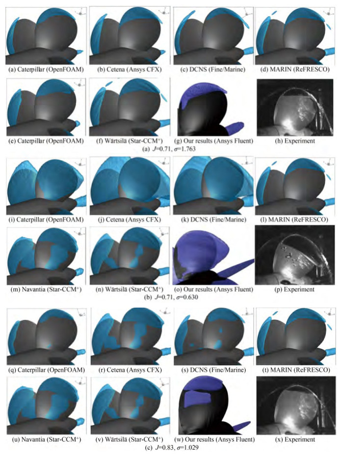Figure  5  The cavitation patterns in comparison with different simulation studies and experiments

Download: Full-Size Img

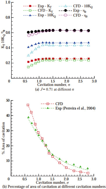Figure  6  Comparison of hydrodynamic performance of the propeller

Download: Full-Size Img

The open-water propeller tests are conducted for six different cavitation numbers. One of them is the non-cavitating case which has a cavitation number of σ = 27.6, while for the other five tests it was σ ≤ 5. The cavitation number in CFD simulations is varied by changing the outlet pressure. All the parameters used in simulations are given in Table 4.

The INSEAN E779A propeller in open-water is forced to cavitate by changing the outlet pressure in the fluid domain. The open-water propeller performance is investigated with changing cavitation numbers. Results of numerical simulations are given in Figure 7.

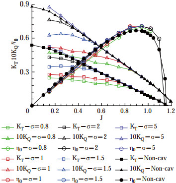Figure  7  Comparison of the open-water propeller performance with different cavitation numbers

Download: Full-Size Img

Except the case of σ = 5, the thrust and torque coefficients are reduced at lower advance ratios. They are similar to the non-cavitating case at higher J. Observing Figure 7 at same (low) advance coefficients, the graph suggests that the thrust coefficient decreases as the cavitation number decreases. This is due to the high loading on the propeller blades: the propeller is compelled to generate thrust under greater cavitation. Similar statements can be made for the torque coefficient. The decrease in the thrust coefficient with respect to increasing cavitation size was also noted in (Gaggero and Villa, 2018). The open-water efficiency is lower at lower advance ratios compared to the non-cavitating case. However; cavitation increases the efficiency at higher J where we normally expect the point of ship self-propulsion. This is considered to be significant because it sheds light on the rare occasion of increased propulsion efficiency despite the cavitation formation.

Figure 8 shows the cavity extent at different cavitation numbers for the same advance coefficient of J = 0.348. The cavity volume increases with a decrease in cavitation number which mainly affect the hydrodynamic performance of the propeller significantly.

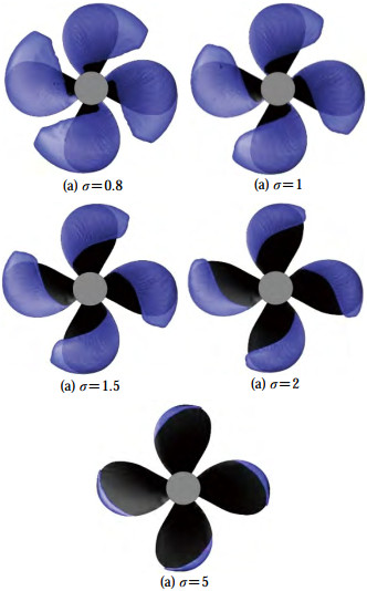Figure  8  Cavity extents for different sigma numbers (J＝0.348, α_v＝0.5)

Download: Full-Size Img

6.2   Calculation results for behind-the-hull condition

The INSEAN E779A propeller considered in this study was also tested in behind-the-ship hull condition and its performance in full-scale KCS (KRISO container ship) self-propulsion condition was assessed. The original propeller of KCS is the KP505 propeller with a diameter of D = 7.9 m; however, in this study we have replaced it with INSEAN E779A propeller of similar size. Despite an increase in the cavitation extent with increasing propeller size (Regener et al., 2018), minor changes at similar advance ratio and cavitation number are reported (Tani et al., 2019). Therefore, the open-water propeller performance obtained at the model scale was used directly without any corrections in K_T and K_Q, as these would have negligible effects on the overall results. Self-propulsion parameters were obtained using the self-propulsion estimation (SPE) method available in (Kinaci et al., 2018) and (Gokce et al., 2019). The geometrical description and main particulars of the full scale KCS (KRISO container ship) are shown in Table 5 and Figure 9.

Figure  9  Geometry of KCS (KRISO container ship)

Download: Full-Size Img

Self-propulsion parameters are to be found for the service speed of this ship which is at V = 24 kn. SPE requires four inputs and these are bare hull total resistance, open-water propeller performance, wake fraction and thrust deduction factor. Values of bare hull total resistance, wake fraction and thrust deduction factor are taken from (Can et al., 2020). The open-water propeller performance of the cavitating INSEAN E779A are taken from the curve-fit equations at different cavitation numbers. The thrust coefficient K_T and the torque coefficientK_Q were defined as functions of the advance ratio J and expressed by second-order polynomials:

Coefficientsk₀, k₁, k₂, g₀, g₁ andg₂ of thrust and torque coefficients depend on the cavitation number and their values are given in Table 6. Self-propulsion parameters with changing cavitation number are given in Figure 10(a). The propeller rotation rates for each case are given in Figure 10(b).

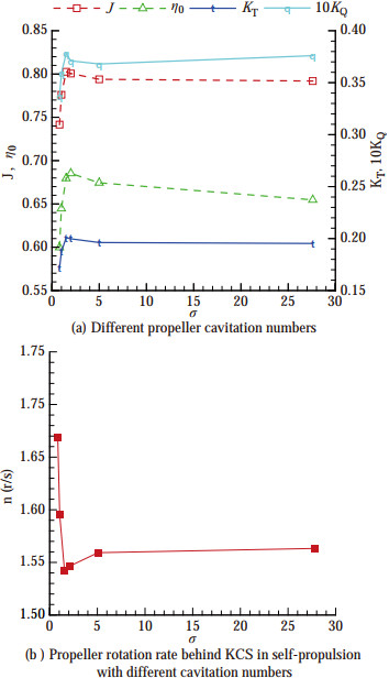Figure  10  The behavior of self-propulsion parameters

Download: Full-Size Img

As Figure 10 suggests, the ship self-propulsion point changes with respect to different cavitation numbers. Cavitation is normally an unwanted phenomenon but it may sometimes enhance the propulsion performance of the ship, under rare circumstances. Here, as is visible in Figure 10(b), the required propeller rotation rate to propel the ship (at the service speed of V = 24 kn) reaches its lowest value at σ = 1.5. The propeller efficiency also makes a peak at this specific cavitation number as well as the thrust and torque coefficients. When the propeller is highly cavitating at cavitation numbers σ < 1.5, the required power to propel the ship will significantly increase as the slope of the propeller rotation rate is significantly high. After σ > 5, changes in the propulsion parameters are monotonic and negligible due to gradually vanishing cavitation.

7   Conclusion

In this study, the open-water performance of INSEAN E779A propeller was investigated under cavitating and non-cavitating conditions. The hydrodynamic performance depends on the cavitation number and the advance ratio of the propeller. In this respect, we followed a test matrix composed of 5 cavitating and 1 non-cavitating cases. For each of these cases, the whole advance ratio range was numerically simulated up to J ≤ 1.2. The implemented grid was selected after sensitivity analysis and by observation of the tip vortex cavitation. Non-cavitating simulations were also performed with this grid. Slight differences with experimental measurements were noted. For the cavitating cases, the formation of sheet cavitation was captured with greater accuracy.

The cavitating simulations showed that cavitation generally reduces the thrust and torque coefficients at lower advance ratios. An exception of this was the case of σ = 5 where we nearly observed a similar propeller performance compared to the non-cavitating case. This is considered to be normal, as the cavitation is about to vanish after this cavitation number.

The subjected propeller was also tested behind the full-scale KCS under self-propulsion conditions to understand the effects of cavitation on ship propulsion. In this respect, we investigated the advance coefficient and the cavitation number domain to graph the changes in thrust and torque coefficients and the propeller efficiency. Changes in the ship self-propulsion point were observed at different cavitation numbers. An interesting condition was encountered at σ = 1.5 where the propulsion performance of the ship was enhanced. The propulsion performance dramatically worsened at lower σ and became gradual (and nearly negligible) after σ > 5. Future studies are planned to simulate the cavitating propeller behind a full-scale ship to assess the total propulsion performance.