Hydrodynamic Performance of a Very Large Floating Structure with Oscillating Water Columns: Semi-analytical Investigation
https://doi.org/10.1007/s11804-023-00331-z
-
Abstract
Responses of the very large floating Structures (VLFS) can be mitigated by implementing oscillating water columns (OWCs). This paper explores the fundamental mechanism of present wave interactions with both structures and examines the hydrodynamic performance of VLFS equipped with OWCs (VLFS-OWCs). Under the linear potential flow theory framework, the semi-analytical model of wave interaction with VLFS-OWCs is developed using the eigenfunction matching method. The semi-analytical model is verified using the Haskind relationship and wave energy conservation law. Results show that the system with dual-chamber OWCs has a wider frequency bandwidth in wave power extraction and hydroelastic response mitigation of VLFS. It is worth noting that the presence of Bragg resonance can be trigged due to wave interaction with the chamber walls and the VLFS, which is not beneficial for the wave power extraction performance and the protection of VLFS.Article Highlights• A semi-analytical model is developed for wave interaction of very large floating structures (VLFS) with oscillating water columns (OWCs);• The response of VLFS is effectively mitigated by implementing OWCs;• The Bragg reflection dominates the influence of the OWCs on the response of VLFS at certain frequencies. -
1 Introduction
Very large floating structures (VLFS) are of great significance from a point of view of exploiting/utilizing ocean space or resources, e.g., the floating airport (Suzuki et al., 2006) and offshore aquaculture engineering (Buck et al., 2018; Chu et al., 2020). Various structures have been patented and investigated widely. Compared with the conventional coastal and offshore foundation (e. g., land-based breakwaters), VLFS possesses some advantages of being mobile, easy to expand and shrink and not affected by sea-level rise (Wang and Wang, 2015).
Unlike the problems of wave interaction with a rigid body, the hydroelasticity of the VLFS shall need to be considered. Greenhill (1886) and Wadhams (1973) pioneered the investigation of wave interaction with elastic bodies. They pointed out that the deformation of the plate shall not be neglected. In addition, the different forms of dispersion relations would appear when waves propagate under elastic plates. Based on Liu et al. (1994) and Wadhams (1973), Li et al. (1999) simplified the dispersion equation of waves in ice-covered waters of infinite length and calculated the deformation of waves after it was introduced into ice-covered waters by using the energy flux method. Evans and Davies (1968) firstly used the Wiener-Hopf method to solve the mixed boundary problem of wave-ice interaction. Fox and Squire (1990) determined the reflection and transmission coefficients by expanding the eigenfunction of the velocity potential and introducing a minimum error function. Kim and Ertekin (1998) replaced the non-orthogonal eigenfunction under the ice layer of Fox and Squire (1990) with orthogonal eigenfunction satisfying dispersion relations, effectively improving the calculation efficiency. Sahoo et al. (2001) introduced a new eigenfunction with orthogonality and extended the solution under simply supported and built-in edge conditions. Teng et al. (2001) optimized the method of Sahoo et al. (2001) to make the coefficient matrices diagonal. Hence, the solution of the associated linear system is particularly simple (Xu and Lu, 2009). Squire(1995, 2007) gave a detailed introduction to the development of wave-ice interaction, especially in mathematical modeling. Recently, numerical models are proposed to calculate the hydroelasticity of the VLFS. Zhang et al. (2019) calculated the kinematic response of a small ice floe and the flexural motion of a sea ice floe under wave action by Smoothed Particle Hydrodynamics (SPH) method. Cheng et al. (2022) optimized the design and layout of an integrated system of modular WEC-type floating breakwaters and a pontoon-type VLFS by the method of hybrid finite element (FE) - boundary element (BE).
The development of marine clean energy can alleviate energy demand and protect the environment. Among various wave energy devices, OWC wave energy converter is considered to be the most successful because of its simple structure and high reliability (Ning et al., 2019). Through theoretical analysis, numerical simulation, and physical experiments, scholars have conducted comprehensive study on the OWC with single-chamber (He et al., 2019; Simonetti and Cappietti, 2021), dual-chamber (Gang et al., 2022; Rezanejad et al., 2021) and multi-chamber (Doyle and Aggidis, 2019; Zheng et al., 2020) in the opening water. Falcão and Henriques (2016), Shalby et al. (2019), and other scholars also reviewed OWC. Compared with single-chamber OWC, the dual-chamber and multi-chamber OWC have larger energy capture width ratio and effective energy extraction bandwidth. Although the energy capture width ratio of OWC has improved, its high construction cost is a problem for commercial applications. Integrated application of wave energy devices and marine structures is an effective solution to reduce construction costs (Zhao et al., 2021; Zhao et al., 2022; John Ashlin et al., 2018). The successful cases of the Mutriku Wave Power Plant (Torre-Enciso et al., 2009) and REWEC3 breakwater (Arena et al., 2013) also confirm the feasibility of integrating OWC devices with marine structures.
From the reliability of VLFS, the motion response is vital. Hence, many scholars proposed the mitigation scheme, such as bottom-mounted breakwaters (Wang et al., 2010), horizontal and vertical plates (Ohta, 1999; Watanabe et al., 2003), submerged horizontal or inclined plates (Mohapatra and Guedes Soares, 2019; Cheng et al., 2016), wave energy converters, etc. As for wave energy converters, Maeda et al. (2000; 2001) first proposed integrating OWC with VLFS. Hong et al. (2006) investigated the hydroelastic responses of VLFS placed behind a reverse T-shape freely floating breakwater with a built-in OWC, it has been shown numerically that the structural deflections of the VLFS can be reduced significantly by a suitably designed reverse T-shape floating breakwater. During the same period, various VLFS-OWC integration schemes were proposed (Crema et al., 2015; Ikoma et al., 2002; Ikoma et al., 2012; Ikoma et al., 2015; Ikoma et al., 2020; Young and Kyoung, 2007). Hong et al. (2007) and Kyoung et al. (2008) illustrated that the energy capture of OWC and the motion response of VLFS are a pair of opposite changes, and the Power Take-Off (PTO) is the key parameter (Wu et al., 2022), which was also found by Ikoma et al. (2018). Hong et al. (2006) studied the influence of OWC independently operated at the weather side of VLFS on the hydrodynamic response of VLFS. In addition, Hong and Hong (2007) considered the articulated connection mode between OWC and VLFS on this basis, to reduce the anchoring cost. OWC in a non-embedded integrated system operates independently and mitigates the response of VLFS through wave energy conversion.
The effect of an OWC device on the VLFS has been investigated by Maeda (2000; 2001) and Hong et al. (2006; 2007). But the interaction of the VLFS and OWC is not revealed fundamentally in terms of the hydrodynamic coefficient and excitation volume flux. Nevertheless, that illustration is helpful in understanding the combination of VLFS and OWC.
The structure of this paper is as follows: In section 2, the semi-analytical solution method of VLFS-OWCs and the definition of hydrodynamic parameters are given. In section 3, the semi-analytical model program is verified by Haskind relationship and energy conservation. In section 4, the effects of integration parameters on hydrodynamic parameters are discussed. Finally, the conclusions are given in section 5.
2 Analytical solutions
2.1 Mathematical formulation
The sketch of dual-chamber VLFS-OWCs system is shown in Figure 1. A global Cartesian coordinate system O−xz is adopted with Oz being vertically upward and Ox being horizontally rightwards. The VLFS is considered to be a semi-infinite elastic plate that extends to the positive x-direction. A dual-chamber OWCs was arranged at the weather side of VLFS in the water of finite depth h. Symbolically, h1, h2, h3 denote the draft of the front-wall, mid-wall, rear-wall, the corresponding thickness is a1, a2, and a3, respectively. d1, d2, d3 represent the breadths of chamber 1, chamber 2, and spacing between the two structures.
 Figure 1 The sketch of dual-chamber VLFS-OWCs system
Under the potential flow theory framework, the fluid flow is described by the complex velocity potential of Φ (x, y, z, t) = Re[ϕ (x, y, z)e−iωt ], where Re[ ] denotes the real part of the variable; ϕ, i, ω, t, represent the space velocity potential, the imaginary unit, the circular frequency of incident waves, and the time. ϕ can be decomposed as the sum of scattering and radiation potentials, i.e.,
$$ \phi=\phi_1+\phi_2 $$ (1) where ϕ1 denotes the scattering potential, and ϕ2 is the radiation potential.
The fluid domain is divided into eight sub-regions, i.e., Ωn (n=1, …, 8). Referring to Figure 1, the fluid regions Ωn (n=1, …, 8) denotes the fluid region in the weather side of the front-wall (x < x1, l, − h < z < 0), beneath the front-wall (x1, l < x < x1, r, −h < z < −h1), between the front-wall and mid-wall (x1, r < x < x2, l, −h < z < 0), beneath the mid-wall (x2, l < x < x2, r, −h < z < −h2), between the mid-wall and rear-wall (x2, r < x < x3, l, − h < z < 0), beneath the rear-wall (x3, l < x < x3, r, −h < z < −h2), between the rear-wall and VLFS (x3, r < x < x4, l, −h < z < 0), and beneath the VLFS (x > x4, l, −h < z < −T), respectively. Symbolically, the velocity potential in Ωn (n=1, …, 8) was expressed as ϕl(n), which represents the relevant scattering potential for ℓ =1 and the radiation potential for ℓ=2. ϕl(n)shall satisfy governing equation, the free surface condition, elastic plate condition, the impetration condition (both seabed and the OWC walls), pressure-forced surface condition inside the OWC chamber, and the far-field condition. For the present problem, the governing equation can be written as:
$$ \frac{\partial^2 \phi}{\partial x^2}+\frac{\partial^2 \phi}{\partial z^2}=0 $$ (2) The boundary conditions for the scattering and radiation potential can be expressed as:
$$ \left\{\begin{array}{l} \frac{\partial \phi_{\ell}^{(n)}}{\partial z}=\frac{\omega^2}{g} \phi_{\ell}^{(n)}+\frac{\mathrm{i} \omega \delta_{j, n}^{\ell}=2}{\rho g}\left(\begin{array}{l} x<x_{1, l}, \text { or } x_{m, r}<x<x_{m+1, l}, \\ z=0, m=1, 2, 3, j=3, 5 \end{array}\right) \\ \frac{\partial \phi_{\ell}^{(n)}}{\partial z}=0 \quad\left(x_{m, l}<x<x_{m, r}, z=-h_m, m=1, 2, 3\right) \\ \left[E I \frac{\partial^4}{\partial x^4}-m_s \omega^2+\rho g\right] \frac{\partial \phi_{\ell}^{(8)}}{\partial z}-\rho \omega^2 \phi_{\ell}^{(8)}=0 \quad\left(\begin{array}{l} x>x_{4, l}, \\ z=-T \end{array}\right) \\ \frac{\partial \phi_{\ell}^{(n)}}{\partial x}=0\left(\begin{array}{c} x=x_{4, l}, -T<z<0 \text { or } x=x_{m, j}, \\ -h_m<z<0, m=1, 2, 3, j=l, r \end{array}\right) \\ \frac{\partial \phi_{\ell}^{(n)}}{\partial z}=0 \quad(-\infty<x<+\infty, z=-h) \\ \phi_{\ell}^{(n)} \text { outgoing:finitevalue }(|x| \rightarrow \infty, n=1, 8) \end{array}\right.$$ (3) where the initial moment I=C3/[12(1−ν2)]; the mass ms=ρsC; C, E, ν, ρs, ρ, and g are respectively the thickness, Young's modulus, the Poisson's ratio, the surface density of the VLFS, the water density, and the gravitational acceleration.
The deformation of the VLFS is subjective to the edge conditions at the left end (x=x4, l, z=−T). There are three typical edge conditions (Sahoo et al., 2001), i.e., free edge, simply supported edge, and built-in edge conditions, which can be mathematically expressed respectively, as
$$ \frac{\partial^4 \phi_{\ell}^{(8)}}{\partial x^3 \partial z}=0 \text { and } \frac{\partial^3 \phi_{\ell}^{(8)}}{\partial x^2 \partial z}=0 $$ (4) $$ \frac{\partial^3 \phi_{\ell}^{(8)}}{\partial x^2 \partial z}=0 \text { and } \frac{\partial \phi_{\ell}^{(8)}}{\partial z}=0 $$ (5) and
$$ \frac{\partial^2 \phi_{\ell}^{(8)}}{\partial x \partial z}=0 \text { and } \frac{\partial \phi_{\ell}^{(8)}}{\partial z}=0 $$ (6) 2.2 Method of solution
By implementing the eigenfunction matching method, the velocity potential corresponding to each sub-region can be written respectively as:
$$ \left\{ \begin{array} {l} & \phi_l^{(1)}=-\frac{\mathrm{ig} A}{\omega}\left(Z_1\left(\kappa_1 z\right) \mathrm{e}^{\mathrm{i} k x}+\sum\limits_\limits{n=1}^{\infty} A_n^{(\ell, 1)} \mathrm{e}^{\kappa_n x} Z_n\left(\kappa_n z\right)\right) \\ & \phi_{\ell}^{(2)}=-\frac{\mathrm{ig} A}{\omega}\left(A_1^{(\ell, 2)} x+A_1^{(\ell, 3)}+\sum\limits_\limits{n=2}^{\infty}\left(\begin{array}{l} A_n^{(\ell, 2)} \mathrm{e}^{-\gamma_{1, n} x} \\ +A_n^{(\ell, 3)} \mathrm{e}^{-\gamma_{1, n} x} \end{array}\right) V_n\left(\gamma_{1, n} z\right)\right) \\ & \phi_{\ell}^{(3)}=-\frac{\mathrm{i} g A}{\omega}\left(\sum\limits_\limits{n=1}^{\infty}\left(\begin{array}{c} A_n^{(\ell, 4)} \mathrm{e}^{-\kappa_n x} \\ +A_n^{(\ell, 5)} \mathrm{e}^{\kappa_n x} \end{array}\right) Z_n\left(\kappa_n z\right)\right)-\frac{\mathrm{i} \delta_{\ell, m}}{\rho \omega}, (m=2, 3) \\ & \phi_{\ell}^{(4)}=-\frac{\operatorname{ig} A}{\omega}\left(A_1^{(\ell, 6)} x+A_1^{(\ell, 7)}+\sum\limits_\limits{n=2}^{\infty}\left(\begin{array}{l} A_n^{(\ell, 6)} \mathrm{e}^{-\gamma_{2, n} x} \\ +A_n^{(\ell, 7)} \mathrm{e}^{\gamma_{2, n} x} \end{array}\right) V_n\left(\gamma_{2, n} z\right)\right) \\ & \phi_{\ell}^{(5)}=-\frac{\mathrm{i} g A}{\omega}\left(\sum\limits_\limits{n=1}^{\infty}\left(\begin{array}{c} A_n^{(\ell, 8)} \mathrm{e}^{-\kappa_n x} \\ +A_n^{(\ell, 9)} \mathrm{e}^{\kappa_n x} \end{array}\right) Z_n\left(\kappa_n z\right)\right)-\frac{\mathrm{i} \delta_{\ell, m}}{\rho \omega}, (m=2, 4) \\ & \phi_{\ell}^{(6)}=-\frac{\mathrm{ig} A}{\omega}\left(\begin{array}{c} A_1^{(\ell, 10)} x+A_1^{(\ell, 11)} \\ +\sum\limits_\limits{n=2}^{\infty}\left(A_n^{(\ell, 10)} \mathrm{e}^{-\gamma_{3,n} x}+A_n^{(\ell, 11)} \mathrm{e}^{\gamma_{3,n} x}\right) V_n\left(\gamma_{3, n} z\right) \end{array}\right) \\ & \phi_{\ell}^{(7)}=-\frac{\mathrm{ig} A}{\omega}\left(\sum\limits_\limits{n=1}^{\infty}\left(A_n^{(\ell, 12)} \mathrm{e}^{-\kappa_n x}+A_n^{(\ell, 13)} \mathrm{e}^{\kappa_n x}\right) Z_n\left(\kappa_n z\right)\right) \\ & \phi_{\ell}^{(8)}=-\frac{\operatorname{ig} A}{\omega}\left(\begin{array}{c} A_0^{(\ell, 14)} \mathrm{e}^{\mathrm{i}\lambda_0 x} U_0\left(\lambda_0 z\right)+\sum\limits_\limits{n=-2}^{-1} A_n^{(\ell, 14)} \mathrm{e}^{-\lambda_n x} U_n\left(\lambda_n z\right) \\ +\sum\limits_\limits{n=1}^{\infty} A_n^{(\ell, 14)} \mathrm{e}^{-\lambda_n x} U_n\left(\lambda_n z\right) \end{array}\right) \\ & \end{array} \right. $$ (7) where An(l, m) are the unknown coefficient to be solved, m=1, 2, …, 14; ℓ=1, 2, 3, 4, and only 3, 4 is taken when calculating the radiation volume flux. A is the incident wave amplitude; the vertical eigenfunction of Zn(κnz), Vn(γj, nz), and Un (λnz) are defined as:
$$ Z_n\left(\kappa_n z\right)=\cos \left[\kappa_n(z+h)\right] /\cos \left(\kappa_n h\right) $$ (8) $$ V_n\left(\gamma_{j, n} z\right)=\left\{\begin{array}{c} \sqrt{2} /2 \quad n=1 \\ \cos \left[\gamma_{j, n}(z+h)\right] /\cos \left[\gamma_{j, n}\left(h-h_j\right)\right] n \geqslant 2 \end{array}\right. $$ (9) and
$$ U_n\left(\lambda_n z\right)=\left\{\begin{array}{c} \cosh \left[\lambda_n(z+h)\right] /\cosh \left[\lambda_n(h-T)\right] n=0 \\ \cos \left[\lambda_n(z+h)\right] /\cos \left[\lambda_n(h-T)\right] n=-2, -1, 1, 2, \ldots \end{array}\right. $$ (10) respectively. The eigenvalues of k and κn (n ≥ 2) satisfied the dispersion relation of ω2 = gktanhkh and ω2 = − gκntanκnh (n ≥ 2), respectively; κ1 =−ik. The eigenvalues γj, n are given by (n−1) π/(h−hj), (j=1, 2, 3; n=2, 3, …). λn are the positive real roots of following dispersion relations of:
$$ \begin{cases}\lambda_0\left(K \lambda_0^4+W\right) \tanh \left[\lambda_0(h-T)\right]=1 & n=0 \\ -\lambda_n\left(K \lambda_n^4+W\right) \tan \left[\lambda_n(h-T)\right]=1 & n=-2, -1, 1, 2, \ldots\end{cases}$$ (11) where K = EI/(ρω2) and W = (ρg − msω2)/(ρω2). The first equation in Eq. (11) has only one positive real root λ0, and the second equation has two complex roots with the form of λ−1=α+i β and λ−2=α−i β (α and β are both positive real numbers). In addition, the second equation also has infinite positive real roots λn (n=1, 2, 3, …). Thus, the first term in ϕl(8)represents propagation-mode flexural-gravity waves, the second term means propagation waves with rapidly decaying amplitudes, and the third term represents a series of evanescent-mode flexural-gravity waves (Guo et al., 2016). Furthermore, the improved Newton iterative method is used to solve complex roots (Wang et al., 2007), which greatly simplifies the process of solving complex roots.
The complex expansion coefficients An(l, 1)~An(l, 14) can be determined using the edge conditions (i. e., Eqs. (4)-(6)), and the continuity conditions for the scattering and radiated spatial potentials (Eq. A(1)). The detailed solving procedure for the case of free edge condition is given in Appendix A. Once the unknown expansion coefficients are determined, the velocity potentials in eight regions and various hydrodynamic quantities can be evaluated.
2.3 Hydrodynamic parameter
2.3.1 Volume flux inside pneumatic chamber
The excitation volume flux can be obtained through an integration of the vertical water velocity, induced by the joint action of the incident and diffracted wave potentials, across the free surface inside the chambers as:
$$ \begin{aligned} Q_m^{\ell} & =\left.\int_\limits{x_{m r}}^{x_{m+1, l}} \frac{\partial\left(\phi_{\ell}^{(2 m+1)}\right)}{\partial z} \mathrm{~d} x\right|_{z=0} \\ & =-\mathrm{i} \omega A\left[\sum\limits_{n=1}^{\infty}\left[\begin{array}{c} A_n^{(\ell, 4 m)} \frac{\mathrm{e}^{-\kappa_n x_{m+1, l}}-\mathrm{e}^{-\kappa_n x_{m, r}}}{-\kappa_n} \\ +A_n^{(\ell, 4 m+1)} \frac{\mathrm{e}_n^{\kappa_n x_{m+1, l}}-\mathrm{e}^{\kappa_n x_{m, r}}}{\kappa_n} \end{array}\right]\right. \end{aligned} $$ (12) where ℓ=1, m=1, 2.
The radiation volume flux can be obtained through an integration of the vertical water velocity, induced by the radiated wave across the free surface inside the chamber as:
$$ \begin{aligned} Q_{m, j}^{\ell} & =\left.\int_\limits{x_{m, r}}^{x_{m+1, l}} \frac{\partial\left(\phi_{\ell}^{(2 j+1)}\right)}{\partial z} \mathrm{~d} x\right|_{z=0} \\ & =-\mathrm{i} \omega A\left[\sum\limits_{n=1}^{\infty}\left(\begin{array}{c} A_n^{(\ell, 4 j)} \frac{\mathrm{e}^{-\kappa_n x_{m+1, l}}-\mathrm{e}^{-\kappa_n x_{m, r}}}{-\kappa_n} \\ +A_n^{(\ell, 4 j+1)} \frac{\mathrm{e}^{\kappa_n x_{m+1, l}}-\mathrm{e}^{\kappa_n x_{m, r}}}{\kappa_n} \end{array}\right)\right] \end{aligned} $$ (13) where Qm, jl is the radiation volume flux of water column m caused by the pressure forced motion of water column j; m=1, 2, j=1, ℓ=3 and m=1, 2, j=2, ℓ=4. At the same time, where cm, j=Re (Qm, jl) and μm, j=Im(Qm, jl) are the socalled radiation conductance and radiation susceptance (Evans and Porter, 1995).
2.3.2 Hydrodynamic efficiency
The pressure vector and the complex amplitude of the total volume flux can be written as:
$$ \begin{gathered} \left\{\left(\left[\begin{array}{ll} c_{11} & c_{12} \\ c_{21} & c_{22} \end{array}\right]+\left[\begin{array}{ll} c_{\mathrm{PTO}}^{(1)} & \\ & c_{\mathrm{PTO}}^{(2)} \end{array}\right]\right)-\mathrm{i}\left(\left[\begin{array}{ll} \mu_{11} & \mu_{12} \\ \mu_{21} & \mu_{22} \end{array}\right]\right.\right. \\ \left.\left.+\left[\begin{array}{ll} \mu_{\mathrm{PTO}}^{(1)} & \\ & \mu_{\mathrm{PTO}}^{(2)} \end{array}\right]\right)\right\}\left[\begin{array}{l} p_1 \\ p_2 \end{array}\right]=\left[\begin{array}{l} Q_1^1 \\ Q_2^1 \end{array}\right] \end{gathered} $$ (14) where n=1, 2, and pn denotes the pressure in the nth chamber, cPTO(n) represents the PTO damping implemented on the nth chamber, μPTO(n) corresponds to the effects of air compressibility, and there can be found following as:
$$ \mu_{\mathrm{PTO}}^{(n)}=\frac{\omega V_n}{c_a^2 \rho_0} $$ (15) where ca is the sound velocity in air, ρ0 is the static air density, and Vn is the initial air volume inside the nth pneumatic chamber, Vn=0.1dnh.
It is difficult to obtain an analytical expression for the optimal PTO damping of a dual-chamber OWCs, but it can be obtained by numerical approximation. Wang (2018) and Wang et al. (2021) introduced the numerical approximation process in detail. In this paper, the PTO damping near the maximum hydrodynamic efficiency is used (He et al., 2019):
$$ c_{\text {PTO }}^{(n)}=\sqrt{c^2+\left(\mu+\mu_{\text {PTO }}^{(n)}\right)^2} $$ (16) which represents the optimal PTO damping of an isolated OWC.
The power output efficiency corresponding to chamber n (n=1, 2) can be expressed as:
$$ P_n=\frac{1}{2} c_{\mathrm{PTO}}^{(n)} p_n^2 $$ (17) The pn can be obtained by solving the equation (14), and the PTO damping of CPTO(n) is chosen as the equaiton (16).
The incident waves power per width can be written as:
$$ P_{\text {incident }}=\frac{\rho g A^2 \omega}{4 k}\left(1+\frac{2 k h}{\sinh 2 k h}\right) $$ (18) The hydrodynamic efficiency corresponding to chamber n (n=1, 2) can be calculated as:
$$ \eta_n=\frac{P_n}{P_{\text {incident }}} $$ (19) The total hydrodynamic efficiency η can be regarded as the sum of ηn.
2.3.3 Reflection and transmission coefficient
The reflection coefficient KR and the transmission coefficient KT of the proposed system can be expressed as:
$$ \left\{\begin{array}{l} K_{\mathrm{R}}=\left|A_1^{(1, 1)}+p_1 A_1^{(3, 1)}+p_2 A_1^{(4, 1)}\right| \\ K_{\mathrm{T}}=\left|A_0^{(1, 14)}+p_1 A_0^{(3, 14)}+p_2 A_0^{(4, 14)}\right| \frac{\lambda_0 \tanh \lambda_0(h-T)}{k \tanh k h} \end{array}\right. $$ (20) 2.3.4 Hydroelastic parameters
The dimensionless vertical displacement of VLFS can be written as:
$$ \zeta=\frac{\mathrm{i}}{\omega}\left|\frac{\partial \phi_1^{(8)}}{\partial z}+p_1 \frac{\partial \phi_3^{(8)}}{\partial z}+p_2 \frac{\partial \phi_4^{(8)}}{\partial z}\right|_{z=-T} $$ (21) The dimensionless strain of the VLFS in this paper, unless otherwise stated, is located at positive infinity and can be written as:
$$ \varepsilon=\frac{c}{2 \omega}\left|\frac{\partial^3 \phi_1^{(8)}}{\partial^2 x \partial z}+p_1 \frac{\partial^3 \phi_3^{(8)}}{\partial^2 x \partial z}+p_2 \frac{\partial^3 \phi_4^{(8)}}{\partial^2 x \partial z}\right|_{z=-T} $$ (22) The dimensionless shear force of the VLFS is:
$$ \tau=\frac{E I}{\rho g d \omega}\left|\frac{\partial^4 \phi_1^{(8)}}{\partial^3 x \partial z}+p_1 \frac{\partial^4 \phi_3^{(8)}}{\partial^3 x \partial z}+p_2 \frac{\partial^4 \phi_4^{(8)}}{\partial^3 x \partial z}\right|_{z=-T} $$ (23) 3 Verification
In this section, we firstly conduct the convergence analysis of the analytical model, and then the verifications are made based on the Haskind relationship and the wave energy flux conversation. Referring to Hong et al. (2006), the fundamental parameters of VLFS-OWCs are fixed as: A=1 m, h=30 m, ρ=1025 kg/m3, g=9.81 m/s2, E=2.06× 10¹¹ Pa, ν =0.3, ρs=7800 kg/m3, I=0.666, T/h=1/15. In the following sections, the hydrodynamic parameters and PTO system are nondimensionalized by
$$ \begin{gathered} \left\{\bar{c}_{i, j}, \bar{\mu}_{i, j}, \bar{c}_{\text {PTO }}^{(n)}, \bar{\mu}_{\text {PTO }}^{(n)}\right\}=\frac{\rho g}{\omega d_1}\left\{c_{i, j}, \mu_{i, j}, c_{\text {PTO }}^{(n)}, \mu_{\text {PTO }}^{(n)}\right\}, \\ \bar{Q}_m^{\ell}=\frac{\left|Q_m^{\ell}\right|}{\omega d_1 A} . \end{gathered} $$ (24) 3.1 Convergence analysis
A convergence analysis is performed for the dual-chamber VLFS-OWCs with a1/h = a2/h=a3/h=1/60, h1/h=h2/h=h3/h=0.1, d1/h=d2/h=1/6, d3/h=0.1, x1, l=0, V1=0.1d1h, V2=0.1d2h. Figure 2 illustrates the impact of truncation number M on KR, KT, c11, c22, μ11, μ22. It can beseen from Figure 2 that the truncation number of 20 presents excellent convergence.
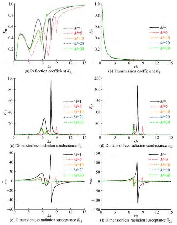 Figure 2 Variations of KR, KT, c11, and μ22 versus the kh with different truncation number M=1, 5, 10, 20, 30
3.2 Haskind relationship
The excitation volume flux can be obtained by integrating the vertical water velocity induced by the joint action of the incident and diffracted wave potentials. This method is regarded as a direct method. In addition, using the Haskind relationship (Haskind, 1957), it can also be calculated based on the far-field radiation waves, which is termed the indirect method. The calculation of the dimensionless excitation volume flux using the direct and indirect method are given by:
$$ \left\{\begin{array}{l} \bar{Q}^{(1)}=\bar{Q}_1^1+\bar{Q}_2^1 \\ \bar{Q}^{(2)}=-\frac{\rho g^2 A^2 A_1^{(2, 1)}\left(\sin \kappa_1 h \cos \kappa_1 h+\kappa_1 h\right)}{\mathrm{i} \omega^2 d_1 A \cos ^2 \kappa_1 h} \end{array}\right. $$ (25) As shown in Figure 3, the dimensionless excitation volume flux calculated by the two different methods agrees well, which may verify the solution of the radiation/diffraction problem.
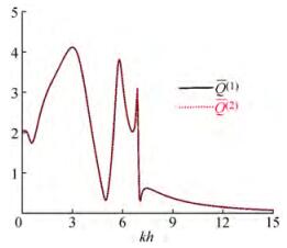 Figure 3 Results of the dimensionless excitation volume flux calculated by the direct and indirect methods
3.3 Wave energy flux conservation
The KR, KT, and η for VLFS-OWCs with dual-chamber are calculated (M=20). From Figure 4, we find that the wave energy flux conservation is satisfied well (i.e., KR2+KT2+η1+η2=1), verifying the semi-analytical model.
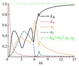 Figure 4 Results of the reflection/transmission coefficient and the hydrodynamic efficiency
4 Results and discussion
The spacing between the OWC structure and the VLFS and edge conditions of the VLFS are two key parameters for the performance of the system. In this section, we explore the influence of the key protesters of OWC damping, edge conditions and spacing on the hydrodynamic performance of the VLFS. The structural/physical parameters of the VLFS-OWCs system are as follows: h = 30 m, a1/h=a2/h=a3/h=1/60, d1/h=d2/h=1/6, d3/h=0.1, h1/h=h2/h=h3/h=0.1, V1=0.1d1h, V2=0.1d2h, x1, l=0.0; ρ =1 025 kg/m3, g=9.81 m/s2, E=2.06×10¹¹ Pa, ν=0.3, ρs=7 800 kg/m3, I=0.666, and T/h=1/15.
4.1 Comparison between the VLFS with and without OWCs
To compare the effect of the number of OWC chambers, both the single- and dual-chamber OWCs are considered here. Note that the breadth of the single-chamber OWC is identical to that of the dual-chamber device. The structural parameters of the single-chamber device are as follows: the thickness of the wall is 1/60 h, the draft of the wall is 0.1 h, the breadth of the chamber is 1/3 h+1/60 h, the spacing between the OWC and VLFS is 0.1 h. Here we balance the hydrodynamic interaction between OWC and VLFS by exploring the characteristics of the reflection coefficient KR, total hydrodynamic efficiency η, transmission coefficient KT, dimensionless strain, dimension less excitation volume flux Q(1), dimensionless radiation conductance c and dimensionless radiation susceptance μ. Figure 5 plots the results of KR, η, KT, ε, Q(1), c and μ as function of kh. Note that the free edge condition of the VLFS is considered.
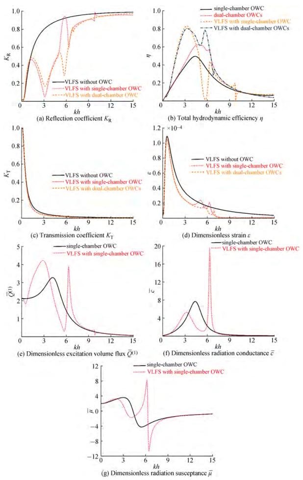 Figure 5 Variations of KR, η, KT, ε, Q(1), c, and μ versus dimensionless wave number kh with and without OWCs
From Figure 5(a), it is found that KR can be reduced by implementing the OWCs on the weather side. Intuitively, it is because the part of incident wave power is absorbed by OWCs (see Figure 5(b)). Therefore, the reflection coefficient curve of the single-chamber OWC and dual-chamber OWCs is of interest. Interestingly, we observe that there exists a peak of KR at kh=5.76 for the VLFS with single-chamber OWC, accounting for the Bragg resonance (Garnaud and Mei, 2009; Zhao et al., 2021), which is caused by the wave interacting with multiple OWC chamber walls and the VLFS structures. However, the wave reflection corresponding to the VLFS with dual-chamber OWCs is relatively milder. KR of VLFS with single-and dual-chamber OWCs has a valley value at kh≈3, which is due to the fact that the peak hydrodynamic efficiency occurs (see Figure 5 (b)).
Figure 5(b) plots the hydrodynamic efficiency of the single- or dual-chamber OWCs with and without the VLFS. It can be found that the VLFS affects the performance of the OWCs significantly, which is mainly reflected in that the η of OWCs increased because of the wave reflection by VLFS. It should be noted that the variation of hydrodynamic efficiency at kh=5.76 is opposite to that of the reflection coefficient. Furthermore, the hydrodynamic efficiency remains 0 while the Bragg resonance is triggered. Notably, the hydrodynamic efficiency of 0 is removed for the VLFS with dual-chamber OWCs, which corresponds to the trend of wave reflection in Figure 5(a).
From Figures 5(c) and (d), we conclude that the presence of the OWCs affects the transmission coefficient slightly. Interestingly, it is found that the strain of the VLFS is significantly reduced due to the shadow effect of the OWCs.
The variation of the Q(1) of the single-chamber OWC with and without VLFS is shown in Figure 5(e), as it can be seen that the Q(1) of OWC with VLFS becomes more complicated. It is worth noting that the peak value of Q(1) appears at kh=6.36, which leads to the peak value of η in Figure 5(b).
Figures 5(f) and (g) show the results of c and μ of single-chamber OWC with and without VLFS. In general, c and μ of single-chamber VLFS-OWC are smaller than that of isolated single-chamber OWC.
In summary, the absorption of wave energy by the OWCs can reduce the KR and of the system. But, adversely, the reflection of wave energy by VLFS can increase the η of OWC. Hence, the hydrodynamic synergies can be produced for the interaction of the OWC and the VLFS with proper design. But attention should be paid to the occurrence of a strong reflection phenomenon, which shall be avoided in the engineering design.
4.2 Effect of the edge conditions of the VLFS
Edge conditions (Guo et al., 2016) affect the hydrodynamic characteristics of the VLFS. Compared with single-chamber OWC in the previous section, dual-chamber OWCs has better advantages in hydrodynamic efficiency and reduction of reflection coefficient. In this section, we investigate the performance of the VLFS with dual-chamber OWCs system with different edge conditions (i. e., free edge, simply supported edge, and built-in edge). The results of the KR, η and corresponding to different edge conditions are shown in Figure 6.
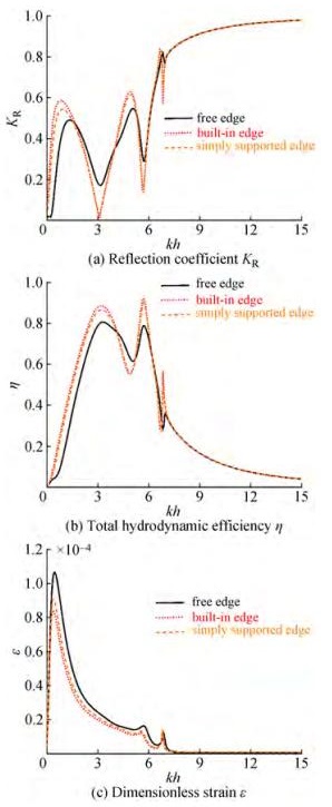 Figure 6 Variations of KR, η, and ε versus dimensionless wave number kh with different edge conditions
In general, the edge condition slightly affects the hydrodynamics of the VLFS-OWCs system. The results corresponding to the conditions of simply supported edge and built-in edge are similar. However, a noticeable difference was observed while comparing the results of the free edge and the built-in edge (or simply supported edge). Notably, the strain of the VLFS is the largest under the condition of free edge. Physically, this shows that the free edge of VLFS is favorable for wave propagation. Teng et al. (2006) demonstrated that the transmission coefficient for the VLFS is most efficient under the free edge.
4.3 Effect of the spacing between the OWCs and VLFS
The spacing dominates the performance of the multi-body system. In this section, we investigate the effect of the spacing between OWCs and the VLFS on the performance of the VLFS-OWCs system. By referring (Hong et al., 2006), Figure 7 shows the KR, η, ε, η1, η2, c11, c12, and c11 + c12 of VLFS-OWCs system for different spacings (i.e., d3/h=0.01, 0.1, 0.2, 0.3). The geometrical/physical parameters are fixed as a1/h=a2/h=a3/h=1/60, d1/h=d2/h=1/6, h1/h=h2/h=h3/h=0.1, V1=0.1d1h, V2=0.1d2h, I=0.666, and T/h=1/15. The free edge condition is used here.
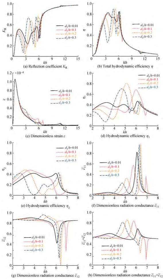 Figure 7 Variations of KR, η, ε, η1, η2, c11, c12, and c11 + c12 versus dimensionless wave number kh with different spacing d3/h=0.01, 0.1, 0.2, 0.3
From Figure 7(a), we found strong oscillations in the range of 0.78 < kh < 6.54 for the reflection coefficient. The spacing dominates the location and the number of oscillations. This is similar to that found in Ning et al. (2017) and Zhao et al. (2021), who paid attention to the effect of the spacing of the multi-pontoon system. As is illustrated in Section 4.1, the strong reflection is attributed to the Bragg resonance. Moreover, the spacing dominated the occurrence of the Bragg resonance.
The trend of η is opposite to that of the KR. Multiple peaks are observed, which corresponds to that the valleys of the reflection coefficient. From the hydrodynamic efficiency curves of chambers 1 and 2 in Figure 7 (d, e), it can be known that the hydrodynamic efficiency peak (d3/h=0.2, kh ≈ 5.1; d3/h= 0.3, kh ≈ 4.7) is triggered by the increment of hydrodynamic efficiency of chamber 1. The radiation conductance reflects the wave energy absorption capacity of OWC, and the amplitude is maximum at this frequency (Figure 7 (h)). The c 12 corresponding to the peak value of hydrodynamic efficiency is positive and maximum, and the hydrodynamic interaction between OWCs shows a positive synergistic effect, which is the main reason for the multi-peak phenomenon.
From Figure 8, it can be found that the KR, η, and KT vary periodically as the spacing between the OWCs and VLFS increases, the dimensionless spacing kd3/π significantly affects the hydrodynamic performance of the system. Sarkar et al. (2015) found that the condition of kd3/π=0.5+n triggered the sloshing resonance in the water region between the wave energy device and the seawall, and the hydrodynamic efficiency showed a valley value. The trigger condition is related to the KR of the seawall and the size of the wave energy device, and there will be a deviation (Zhao et al., 2021). It is worth noting that the triggering conditions of sloshing resonance in the water region between OWCs and VLFS are different under different kh, but the variation periods of KR, η, and KT are kd3/π=1, which is because the reflection effect of VLFS changes with the change of kh.
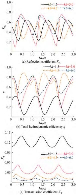 Figure 8 KR, η, and ε versus dimensionless spacing kd3/π with different dimensionless wave number kh
In summary, the spacing imposes an impact on the reflection coefficient and efficiency. However, the spacing between the OWCs and VLFS affects the strain of the VLFS slightly. The spacing is the key parameter for the hydrodynamic performance of VLFS-OWCs, so it should befully considered in engineering design.
5 Conclusions
The matching eigenfunction expansion method is applied to investigate wave interaction with VLFS-OWCs. This method is validated by the Haskind relationship and energy conservation. Then, the interaction between waves and VLFS-OWCs is discussed extensively. The following
conclusions could be drawn:
1) VLFS-OWCs have a lower KR, KT, and in the frequency range of ordinary compared to VLFS, mainly due to the wave energy conversion of OWC.
2) Compared with OWC, VLFS-OWCs have a higher η, and this effect gain is more effective for dual-chamber OWC. This is because the wave energy reflected by VLFS increases the η of OWC.
3) Bragg resonances are triggered by the single-chamber VLFS-OWC, caused by the wave interacting with multiple OWC chamber walls and the VLFS.
4) The minimum of OWC and the maximum η of VLFS appear when the left end of VLFS is under the free edge because the free motion of the VLFS ends has the most negligible effect on wave propagation.
5) Compared with OWC without VLFS, the η and KR of VLFS-OWCs demonstrate multiple peaks. This is mainly due to the hydrodynamic interaction between the two OWCs.
Appendix A
We will use pressure continuity and velocity continuity to determine the unknown coefficients. The continuity conditions of scattering and radiation space potential are as follows:
$$ \frac{\partial \phi_{\ell}^{(2 m-1)}}{\partial x}=\left\{\begin{array}{c} 0 \quad\left(x=x_{m, l}, -h_m<z<0\right) \\ \frac{\partial \phi_{\ell}^{(2 m)}}{\partial x}\left(x=x_{m, l}, -h<z<-h_m\right) \end{array}, m=1, 2, 3\right. $$ (A(1)) $$ \frac{\partial \phi_{\ell}^{(2 m+1)}}{\partial x}=\left\{\begin{array}{c} 0 \quad\left(x=x_{m, r}, -h_m<z<0\right) \\ \frac{\partial \phi_{\ell}^{(2 m)}}{\partial x}\left(x=x_{m, r}, -h<z<-h_m\right) \end{array}, m=1, 2, 3\right. $$ (A(2)) $$ \frac{\partial \phi_{\ell}^{(7)}}{\partial x}=\left\{\begin{array}{c} 0 \quad\left(x=x_{4, l}, -T<z<0\right) \\ \frac{\partial \phi_{\ell}^{(8)}}{\partial x}\left(x=x_{4, l}, -h<z<-T\right) \end{array}\right. $$ (A(3)) $$ \phi_{\ell}^{(2 m-1)}=\phi_{\ell}^{(2 m)} \quad x=x_{m, l}, -h<z<-h_m, m=1, 2, 3 $$ (A(4)) $$ \phi_{\ell}^{(2 m)}=\phi_{\ell}^{(2 m+1)} \quad x=x_{m, r}, -h<z<-h_m, m=1, 3, 3 $$ (A(5)) $$ \phi_{\ell}^{(7)}=\phi_{\ell}^{(8)} \quad x=x_{4, l}, -h<z<-T $$ (A(6)) We make use of the orthogonality of both trigonometric functions and vertical eigenfunction to obtain the equation system with M. Together with the application of the velocity continuity conditions, we have:
$$ \begin{aligned} & \int_\limits{-h}^0\left(\mathrm{i} k Z_1\left(\kappa_1 z\right) \mathrm{e}^{\mathrm{i} k x}+\sum\limits_{n=1}^{\infty} A_n^{(\ell, 1)} \kappa_n{ }^{\kappa_n x} Z_n\left(\kappa_n z\right)\right) Z_m\left(\kappa_m z\right) \mathrm{d z}\\ & =\int_\limits{-h}^{-h_1}\left(A_1^{(\ell, 2)}+\sum\limits_{n=2}^{\infty}\left(-\gamma_{1, n} A_n^{(\ell, 2)} \mathrm{e}^{-\gamma_{1, n, x}}+\gamma_{1, n} A_n^{(\ell, 3)} \mathrm{e}^{\gamma_{1, n} x}\right) V_n\left(\gamma_{1, n} z\right)\right) \\ & Z_m\left(\kappa_m z\right) \mathrm{d} z \text { at } x=x_{1, l} \end{aligned} $$ (A(7)) $$ \begin{aligned} & \int_\limits{-h}^{-h_1}\left\{A_1^{(\ell, 2)}+\sum\limits_{n=2}^{\infty}\left(-\gamma_{1, n} A_n^{(\ell, 2)} \mathrm{e}^{-\gamma_{1, n} x}+\gamma_{1, n} A_n^{(\ell, 3)} \mathrm{e}^{\gamma_{1, n} x}\right) V_n\left(\gamma_{1, n} z\right)\right\} \\ & Z_m\left(\kappa_m z\right) \mathrm{d} z=\int_\limits{-h}^0\left\{\sum\limits_{n=1}^{\infty}\left(-\kappa_n A_n^{(\ell, 4)} \mathrm{e}^{-\kappa_n x}+\kappa_n A_n^{(\ell, 5)} \mathrm{e}^{\kappa_n x}\right) Z_n\left(\kappa_n z\right)\right\} \\ & Z_m\left(\kappa_m z\right) \mathrm{d} z \text { at } x=x_{1, r} \end{aligned} $$ (A(8)) $$ \begin{aligned} & \int_\limits{-h}^0\left\{\sum\limits_{n=1}^{\infty}\left(-\kappa_n A_n^{(\ell, 4)} \mathrm{e}^{-\kappa_n x}+\kappa_n A_n^{(\ell, 5)} \mathrm{e}^{\kappa_n x}\right) Z_n\left(\kappa_n z\right)\right\} Z_m\left(\kappa_m z\right) \mathrm{d} z \\ & =\int_\limits{-h}^{-h_2}\left\{A_1^{(\ell, 6)}+\sum\limits_{n=2}^{\infty}\left(-\gamma_{2, n} A_n^{(\ell, 6)} \mathrm{e}^{-\gamma_{2, n,} x}+\gamma_{2, n} A_n^{(\ell, 7)} \mathrm{e}^{\gamma_{2, n, } x}\right) V_n\left(\gamma_{2, n} z\right)\right\} \\ & Z_m\left(\kappa_m z\right) \mathrm{d} z \text { at } x=x_{2, l} \end{aligned} $$ (A(9)) $$ \begin{aligned} & \int_\limits{-h}^{-h_2}\left\{A_1^{(\ell, 6)}+\sum\limits_{n=2}^{\infty}\left(-\gamma_{2, n} A_n^{(\ell, 6)} \mathrm{e}^{-\gamma_{2, n} x}+\gamma_{2, n} A_n^{(\ell, 7)} \mathrm{e}^{\gamma_{2, n} x}\right) V_n\left(\gamma_{2, n} z\right)\right\} \\ & Z_m\left(\kappa_m z\right) \mathrm{d} z=\int_\limits{-h}^0\left\{\sum\limits_{n=1}^{\infty}\left(-\kappa_n A_n^{(\ell, 8)} \mathrm{e}^{-\kappa_n x}+\kappa_n A_n^{(\ell, 9)} \mathrm{e}^{\kappa_n x}\right) Z_n\left(\kappa_n z\right)\right\} \\ & Z_m\left(\kappa_m z\right) \mathrm{d} z \text { at } x=x_{2, r} \end{aligned} $$ (A(10)) $$ \begin{aligned} & \int_\limits{-h}^0\left\{\sum\limits_{n=1}^{\infty}\left(-\kappa_n A_n^{(\ell, 8)} \mathrm{e}^{-\kappa_n x}+\kappa_n A_n^{(\ell, 9)} \mathrm{e}^{\kappa_n x}\right) Z_n\left(\kappa_n z\right)\right\} Z_m\left(\kappa_m z\right) \mathrm{d} z \\ & =\int_\limits{-h}^{-h_3}\left\{A_1^{(\ell, 10)}+\sum\limits_{n=2}^{\infty}\left(-\gamma_{3, n} A_n^{(\ell, 10)} \mathrm{e}^{-\gamma_{3, n} x}+\gamma_{3, n} A_n^{(\ell, 11)} \mathrm{e}^{\gamma_{3, n} x}\right) V_n\left(\gamma_{3, n} z\right)\right\} \\ & Z_m\left(\kappa_m z\right) \mathrm{d} z \text { at } x=x_{3, l} \end{aligned} $$ (A(11)) $$ \begin{aligned} & \int_\limits{-h}^{-h_3}\left\{A_1^{(\ell, 10)}+\sum\limits_{n=2}^{\infty}\left(-\gamma_{3, n} A_n^{(\ell, 10)} \mathrm{e}^{-\gamma_{3, n} x}+\gamma_{3, n} A_n^{(\ell, 11)} \mathrm{e}^{\gamma_{3, n} x}\right) V_n\left(\gamma_{3, n} z\right)\right\} \\ & Z_m\left(\kappa_m z\right) \mathrm{d} z=\int_\limits{-h}^0\left\{\sum\limits_{n=1}^{\infty}\left(-\kappa_n A_n^{(\ell, 12)} \mathrm{e}^{-\kappa_n x}+\kappa_n A_n^{(\ell, 13)} \mathrm{e}^{\kappa_n x}\right) Z_n\left(\kappa_n z\right)\right\} \\ & Z_m\left(\kappa_m z\right) \mathrm{d} z \text { at } x=x_{3, r} \end{aligned} $$ (A(12)) $$ \begin{aligned} & \int_\limits{-h}^0\left\{\sum\limits_{n=1}^{\infty}\left(-\kappa_n A_n^{(\ell, 12)} \mathrm{e}^{-\kappa_n x}+\kappa_n A_n^{(\ell, 13)} \mathrm{e}^{\kappa_n x}\right) Z_n\left(\kappa_n z\right)\right\} Z_m\left(\kappa_m z\right) \mathrm{d} z \\ & =\int_\limits{-h}^{-T}\left\{{i} \lambda_0 \mathrm{e}^{\mathrm{i} \lambda_0 x} A_0^{(\ell, 14)} U_0\left(\lambda_0 z\right)-\lambda_n \mathrm{e}-\sum\limits_{n=-2}^{-1} A_n^{(\ell, 14)} U_n\left(\lambda_n z\right)\right. \\ & \left.-\lambda_n \mathrm{e}^{-\lambda_n x} \sum\limits_{n=1}^{\infty} A_n^{(\ell, 14)} U_n\left(\lambda_n z\right)\right\} Z_m\left(\kappa_m z\right) \mathrm{d} z \text { at } x=x_{4, l} \end{aligned} $$ (A(13)) Similarly, together with the application of the pressure continuity conditions, we have:
$$ \begin{aligned} & \int_\limits{-h}^{-h_1}\left(Z_1\left(\kappa_1 z\right) \mathrm{e}^{\mathrm{i} k x}+\sum\limits_{n=1}^{\infty} A_n^{(\ell, 1)} \mathrm{e}^{\kappa_n x} Z_n\left(\kappa_n z\right)\right) V_m\left(\gamma_{1, m} z\right) \mathrm{d} z \\ & =\int_\limits{-h}^{-h_1}\left\{A_1^{(\ell, 2)} x+A_1^{(\ell, 3)}+\sum\limits_{n=2}^{\infty}\left(A_n^{(\ell, 2)} \mathrm{e}^{-\gamma_{1, n} x}+A_n^{(\ell, 3)} \mathrm{e}^{\gamma_{1, n} x}\right) V_n\left(\gamma_{1, n} z\right)\right\} \\ & V_m\left(\gamma_{1, m} z\right) \mathrm{d} z \text { at } x=x_{1, l} \end{aligned} $$ (A(14)) $$ \begin{aligned} & \int_\limits{-h}^{-h_1}\left\{A_1^{(\ell, 2)} x+A_1^{(\ell, 3)}+\sum\limits_{n=2}^{\infty}\left(A_n^{(\ell, 2)} \mathrm{e}^{-\gamma_{1, n} x}+A_n^{(\ell, 3)} \mathrm{e}^{\gamma_{1, n} x}\right) V_n\left(\gamma_{1, n} z\right)\right\} \\ & V_m\left(\gamma_{1, m} z\right) \mathrm{d} z=\int_\limits{-h}^{-h_1}\left\{\sum\limits_{n=1}^{\infty}\left(A_n^{(\ell, 4)} \mathrm{e}^{-\kappa_n x}+A_n^{(\ell, 5)} \mathrm{e}^{\kappa_n x}\right) Z_n\left(\kappa_n z\right)+\frac{\delta_{\ell, 2}}{\rho g A}\right\} \\ & V_m\left(\gamma_{1, m} z\right) \mathrm{d} z \text { at } x=x_{1, r} \end{aligned} $$ (A(15)) $$ \begin{aligned} & \int_\limits{-h}^{-h_2}\left\{\sum\limits_{n=1}^{\infty}\left(A_n^{(\ell, 4)} \mathrm{e}^{-\kappa_n x}+A_n^{(\ell, 5)} \mathrm{e}^{\kappa_n x}\right) Z_n\left(\kappa_n z\right)+\frac{\delta_{\ell, 2}}{\rho g A}\right\} V_m\left(\gamma_{2, m} z\right) \mathrm{d} z \\ & =\int_\limits{-h}^{-h_2}\left\{A_1^{(\ell, 6)} x+A_1^{(\ell, 7)}+\sum\limits_{n=2}^{\infty}\left(A_n^{(\ell, 6)} \mathrm{e}^{-\gamma_{2, n} x}+A_n^{(\ell, 7)} \mathrm{e}^{\gamma_{2, n} x}\right) V_n\left(\gamma_{2, n} z\right)\right\} \\ & V_m\left(\gamma_{2, m} z\right) \mathrm{d} z \text { at } x=x_{2, l} \end{aligned} $$ (A(16)) $$ \begin{aligned} & \int_\limits{-h}^{-h_2}\left\{A_1^{(\ell, 6)} x+A_1^{(\ell, 7)}+\sum\limits_{n=2}^{\infty}\left(A_n^{(\ell, 6)} \mathrm{e}^{-\gamma_{2, n} x}+A_n^{(\ell, 7)} \mathrm{e}^{\gamma_{2, n} x}\right) V_n\left(\gamma_{2, n} z\right)\right\} \\ & V_m\left(\gamma_{2, m} z\right) \mathrm{d} z=\int_\limits{-h}^{-h_2}\left\{\sum\limits_{n=1}^{\infty}\left(A_n^{(\ell, 8)} \mathrm{e}^{-\kappa_n x}+A_n^{(\ell, 9)} \mathrm{e}^{\kappa_n x}\right) Z_n\left(\kappa_n z\right)+\frac{\delta_{\ell, 2}}{\rho g A}\right\} \\ & V_m\left(\gamma_{2, m} z\right) \mathrm{d} z \text { at } x=x_{2, r} \end{aligned} $$ (A(17)) $$ \begin{aligned} & \int_\limits{-h}^{-h_3}\left\{\sum\limits_{n=1}^{\infty}\left(A_n^{(\ell, 8)} \mathrm{e}^{-\kappa_n x}+A_n^{(\ell, 9)} \mathrm{e}^{\kappa_n x}\right) Z_n\left(\kappa_n z\right)+\frac{\delta_{\ell, 2}}{\rho g A}\right\} V_m\left(\gamma_{3, m} z\right) \mathrm{d} z \\ & =\int_\limits{-h}^{-h_3}\left\{A_1^{(\ell, 10)} x+A_1^{(\ell, 11)}+\sum\limits_{n=2}^{\infty}\left(A_n^{(\ell, 10)} \mathrm{e}^{-\gamma_{3, n} x}+A_n^{(\ell, 11)} \mathrm{e}^{\gamma_{3, } x}\right) V_n\left(\gamma_{3, n} z\right)\right\} \\ & V_m\left(\gamma_{3, m} z\right) \mathrm{d} z \text { at } x=x_{3, l} \end{aligned} $$ (A(18)) $$ \begin{aligned} & \int_\limits{-h}^{-h_3}\left\{A_1^{(\ell, 10)} x+A_1^{(\ell, 11)}+\sum\limits_{n=2}^{\infty}\left(A_n^{(\ell, 10)} \mathrm{e}^{-\gamma_{3, n} x}+A_n^{(\ell, 11)} \mathrm{e}^{\gamma_{3, n} x}\right) V_n\left(\gamma_{3, n} z\right)\right\} \\ & V_m\left(\gamma_{3, m} z\right) \mathrm{d} z=\int_\limits{-h}^{-h_3}\left\{\sum\limits_{n=1}^{\infty}\left(A_n^{(\ell, 12)} \mathrm{e}^{-\kappa_n x}+A_n^{(\ell, 13)} \mathrm{e}^{\kappa_n x}\right) Z_n\left(\kappa_n z\right)\right\} \\ & V_m\left(\gamma_{3, m} z\right) \mathrm{d} z \text { at } x=x_{3, r} \end{aligned} $$ (A(19)) $$ \begin{aligned} & \int_\limits{-h}^{-T}\left\{\sum\limits_{n=1}^{\infty}\left(A_n^{(\ell, 12)} \mathrm{e}^{-\kappa_n x}+A_n^{(\ell, 13)} \mathrm{e}^{\kappa_n x}\right) Z_n\left(\kappa_n z\right)\right\} U_m\left(\lambda_m z\right) \mathrm{d} z \\ & =\int_\limits{-h}^{-T}\left\{\left(A_0^{(\ell, 14)} \mathrm{e}^{\mathrm{i} \lambda_0 x}\right) U_0\left(\lambda_0 z\right)+\sum\limits_{n=-2}^{-1}\left(A_n^{(\ell, 14)} \mathrm{e}^{-\lambda_n x}\right) U_n\left(\lambda_n z\right)\right. \\ & \left.+\sum\limits_{n=1}^{\infty}\left(A_n^{(\ell, 14)} \mathrm{e}^{-\lambda_n x}\right) U_n\left(\lambda_n z\right)\right\} U_m\left(\lambda_m z\right) \mathrm{d} z \text { at } x=x_{4, l} \end{aligned} $$ (A(20)) In general, we truncate n and m in equations A(7) -A (20) after M. Special attention is required to truncate m after M-2 in the equation of A(20), combined with the free edge. We obtain and solve a system of 14M+2 linear equations with 14M+2 unknown coefficients.
We also use the same way to determine the velocity potentials for the cases of the VLFS with the simply supported edge and the built-in edge.
Competing interest The authors have no competing interests to declare that are relevant to the content of this article. -
Figure 1 The sketch of dual-chamber VLFS-OWCs system
Figure 2 Variations of KR, KT, c11, and μ22 versus the kh with different truncation number M=1, 5, 10, 20, 30
Figure 3 Results of the dimensionless excitation volume flux calculated by the direct and indirect methods
Figure 4 Results of the reflection/transmission coefficient and the hydrodynamic efficiency
Figure 5 Variations of KR, η, KT, ε, Q(1), c, and μ versus dimensionless wave number kh with and without OWCs
Figure 6 Variations of KR, η, and ε versus dimensionless wave number kh with different edge conditions
Figure 7 Variations of KR, η, ε, η1, η2, c11, c12, and c11 + c12 versus dimensionless wave number kh with different spacing d3/h=0.01, 0.1, 0.2, 0.3
Figure 8 KR, η, and ε versus dimensionless spacing kd3/π with different dimensionless wave number kh
-
Arena F, Romolo A, Malara G, Ascanelli A (2013) On design and building of a U-OWC wave energy converter in the Mediterranean Sea: A case study. ASME 2013 32nd International Conference on Ocean, Offshore and Arctic Engineering. https://doi.org/10.1115/OMAE2013-11593 Buck BH, Troell MF, Gesche K, Angel DL, Britta G, Thierry C (2018) State of the Art and Challenges for Offshore Integrated Multi-Trophic Aquaculture (IMTA). Frontiers in Marine Science, 5, 165. https://doi.org/10.3389/fmars.2018.00165 Cheng Y, Ji C, Zhai G, Oleg G (2016) Dual inclined perforated antimotion plates for mitigating hydroelastic response of a VLFS under wave action. Ocean Engineering, 121: 572-591. https://doi.org/10.1016/j.oceaneng.2016.05.044 Cheng Y, Xi C, Dai S, Ji C, Collu M, Li M, Yuan Z, Incecik A (2022)Wave energy extraction and hydroelastic response reduction of modular floating breakwaters as array wave energy converters integrated into a very large floating structure. Applied Energy, 306: 117953. https://doi.org/10.1016/j.apenergy.2021.117953 Chu YI, Wang CM, Park JC, Lader PF (2020) Review of cage and containment tank designs for offshore fish farming. Aquaculture, 519: 734928. https://doi.org/10.1016/j.aquaculture.2020.734928 Crema I, Simonetti I, Cappietti L, Oumeraci H (2015) Laboratory experiments on oscillating water column wave energy converters integrated in a very large floating structure. 11th European Wave and Tidal Energy Conference, EWTEC 2015 Doyle S, Aggidis GA (2019) Development of multi-oscillating water columns as wave energy converters. Renewable and Sustainable Energy Reviews, 107: 75-86. https://doi.org/10.1016/j.rser.2019.02.021 Evans DV, Davies TV (1968) Wave-Ice Interaction. Davidson Laboratory, Stevens Institute of Technology, Hoboken Evans DV, Porter R (1995) Hydrodynamic characteristics of an oscillating water column device. Applied Ocean Research, 17(3): 155-164. https://doi.org/10.1016/0141-1187(95)00008-9 Falcão AFO, Henriques JCC (2016) Oscillating-water-column wave energy converters and air turbines: A review. Renewable Energy, 85: 1391-1424. https://doi.org/10.1016/j.renene.2015.07.086 Fox C, Squire VA (1990) Reflection and transmission characteristics at the edge of shore fast sea ice. Journal of Geophysical Research, 95(7): 11629-11639. https://doi.org/10.1029/JC095iC07p11629 Gang A, Guo B, Hu Z, Hu R (2022) Performance analysis of a coastOWC wave energy converter integrated system. Applied Energy. 311, 118605. https://doi.org/10.1016/j.apenergy.2022.118605 Garnaud X, Mei CC (2009) Bragg scattering and wave-power extraction by an array of small buoys. Proceedings of the Royal Society A: Mathematical, Physical and Engineering Sciences, 466(2113): 79-106. https://doi.org/10.1098/rspa.2009.0458 Greenhill AG (1886) Wave motion in hydrodynamics. American Journal of Mathematics, 9(1): 62-96. https://doi.org/10.2307/2369499 Guo YX, Liu Y, Meng X (2016) Oblique wave scattering by a semiinfinite elastic plate with finite draft floating on a step topography. Acta Oceanologica Sinica, 35(7): 113-121. https://doi.org/10.1007/s13131-015-0760-2 Haskind MD (1957) The exciting forces and wetting of ships in waves. Izvestia Akademii Nauk SSSR Otdelenie Tekhnicheskikh Nauk, (7): 65-79 http://citeseerx.ist.psu.edu/viewdoc/download?doi=10.1.1.892.7434&rep=rep1&type=pdf He F, Zhang HS, Zhao JJ, Zheng SM, Iglesias G (2019) Hydrodynamic performance of a pile-supported OWC breakwater: An analytical study. Applied Ocean Research, 88: 326-340. https://doi.org/10.1016/j.apor.2019.03.022 Hong DC, Hong SY (2007) Hydroelastic responses and drift forces of a very-long floating structure equipped with a pin-connected oscillating-water-column breakwater system. Ocean Engineering, 34(5-6): 696-708. https://doi.org/10.1016/j.oceaneng.2006.05.004 Hong DC, Hong SY, Hong SW (2006) Reduction of hydroelastic responses of a very-long floating structure by a floating oscillatingwater-column breakwater system. Ocean Engineering. 33(5-6): 610-634. https://doi.org/10.1016/j.oceaneng.2005.06.005 Ikoma T, Furuya S, Aida Y, Masuda K, Eto H (2020) Characteristics of OWC type WEC dampers installed on a very large floating structure. ASME 2020 39th International Conference on Ocean, Offshore and Arctic Engineering. https://doi.org/10.1115/omae2020-19002 Ikoma T, Maeda H, Masuda K, Rheem CK, Arita M (2002) Effects of submerged vertical plates and air chamber units in hydroelastic response reductions. 12th International Offshore and Polar Engineering Conference, Kitakyushu, Japan Ikoma T, Masuda K, Rheem CK, Maeda H, Watanabe Y (2012) Primary conversion efficiency of OWC type WECs installed on a large floating structure. ASME 2012 31st International Conference on Ocean, Offshore and Arctic Engineering, Rio de Janerio, Brazil. https://doi.org/10.1115/omae2012-83337 Ikoma T, Masuda K, Watanabe Y, Eto H, Kinoshita T (2015) Power Generation Potential of a VLFS Equipped with OWC Type WECs and Damper Effects on Elastic Motion. ASME 2015 34th International Conference on Ocean, Offshore and Arctic Engineering. https://doi.org/10.1115/omae2015-41960 Ikoma T, Yuka W, Eto H, Masuda K, Omura K (2018) PTO and elastic motion of VLFSs installed with OWC type WECs. OCEANS-MTS/IEEE Kobe Techno-Oceans, Kobe, Japan. https://doi.org/10.1109/oceanskobe.2018.8559273 John Ashlin S, Sannasiraj SA, Sundar V (2018) Performance of an array of oscillating water column devices integrated with an offshore detached breakwater. Ocean Engineering, 163: 518-532. https://doi.org/10.1016/j.oceaneng.2018.05.043 Kim JW, Ertekin RC (1998) An eigenfunction-expansion method for predicting hydroelastic behavior of a shallow-draft VLFS. Proceedings of the 2nd International Conference on Hydroelasticity in Marine Technology, Kyushu University, Fukuoka, Japan Kyoung JH, Hong SY (2008) Localized finite element method on hydroelastic responses of OWC-Embedded VLFS. ASME 2008 27th International Conference on Offshore Mechanics and Arctic Engineering. https://doi.org/10.1115/omae2008-57995 Li CH, Wang YX, Qiu DH (1999) The deformation of wave travelling into water covered by ice. China Offshore Platform, (2): 10-14 http://en.cnki.com.cn/Article_en/CJFDTOTAL-ZGHY199902006.htm Liu XD, Hirayama K, Sakai S (1994) Third order solution wave motion under ice sheet. Marine Offshore & Ice Technology, 383-392. https://doi.org/10.2495/CMO940381 Maeda H, Onishi Y, Rheem CK, Ikoma T, Washio Y, Osawa H, Arita M (2000) Flexible response reduction on a very large floating structure due to OWC wave power devices. Journal of the Japan Society of Naval Architects & Ocean Engineers, 188(188): 279-285. https://doi.org/10.2534/JJASNAOE1968.2000.188_279 Maeda H, Rheem CK, Ikoma T, Masuda K, Fujita N (2001) An experimental study on hydroelastic responses of elastic floating bodies with air chambers in irregular waves. Journal of the Japan Society of Naval Architects & Ocean Engineers, 2001(190): 387-393. https://doi.org/10.2534/jjasnaoe1968.2001.190_387 Mohapatra SC, Guedes Soares C (2019) Interaction of ocean waves with floating and submerged horizontal flexible structures in three-dimensions. Applied Ocean Research, 83: 136-154. https://doi.org/10.1016/j.apor.2018.10.009 Ning D, Wang R, Chen L, Sun K (2019) Experimental investigation of a land-based dual-chamber OWC wave energy converter. Renewable and Sustainable Energy Reviews, 105: 48-60. https://doi.org/10.1016/j.rser.2019.01.043 Ning D, Zhao X, Zhao M, Hann M, Kang H (2017) Analytical investigation of hydrodynamic performance of a dual pontoon WEC-type breakwater. Applied Ocean Research, 65: 102-111. https://doi.org/10.1016/j.apor.2017.03.012 Ohta K (1999) Effect of attachment of a horizontal/vertical plate on the wave response of a VLFS. Proceedings of the Third International Workshop on Very Large Floating Structure, University of Hawaii at Manao Honolulu Rezanejad K, Gadelho JFM, Xu S, Guedes Soares C (2021) Experimental investigation on the hydrodynamic performance of a new type floating oscillating water column device with dual-chambers. Ocean Engineering, 234: 109307. https://doi.org/10.1016/j.oceaneng.2021.109307 Sahoo T, Yip TL, Chwang AT (2001) Scattering of surface waves by a semi-infinite floating elastic plate. Physics of Fluids, 13(11): 3215-3222. https://doi.org/10.1063/1.1408294 Sarkar D, Renzi E, Dias F (2015) Effect of a straight coast on the hydrodynamics and performance of the oscillating wave surge converter. Ocean Engineering, 105: 25-32. https://doi.org/10.1016/j.oceaneng.2015.05.025 Shalby M, Dorrell DG, Walker P (2019) Multi-chamber oscillating water column wave energy converters and air turbines: a review. International Journal of Energy Research, 43(2): 681-696. https://doi.org/10.1002/er.4222 Simonetti I, Cappietti L (2021) Hydraulic performance of oscillating water column structures as anti-reflection devices to reduce harbour agitation. Coastal Engineering, 165: 103837 https://doi.org/10.1016/j.coastaleng.2020.103837 Squire VA (1995) Of ocean waves and sea ice. Annual Review of Fluid Mechanics, 27: 115-168. https://doi.org/10.1146/annurev.fl.27.010195.000555 Squire VA (2007) Of ocean waves and sea-ice revisited. Cold Regions Science and Technology, 49(2): 110-133. https://doi.org/10.1016/j.coldregions.2007.04.007 Suzuki H, Bhattacharya B, Fujikubo M, Hudson DA, Riggs HR, Seto H, Shin H, Shugar TA, Yasuzawa Y, Zong Z (2006) Very large floating structures. 16th International Ship and Offshore Structures Congress, Southampton, UK Teng B, Cheng L, Liu SX, Li FJ (2001) Modified eigenfunction expansion methods for interaction of water waves with a semiinfinite elastic plate. Applied Ocean Research, 6(23): 357-368. https://doi.org/10.1016/S0141-1187(02)00005-6 Teng B, Gou Y, Cheng L, Liu SX (2006) Draft effect on wave action with a semi-infinite elastic plate. Acta Oceanologica Sinica, 25(6). https://doi.org/116-127.10.1016/j.marchem.2005.09.003 Torre-Enciso Y, Ortubia I, de Aguileta LIL, Marqués J (2009) Mutriku wave power plant: from the thinking out to the reality. Proceedings of the 8th European Wave and Tidal Energy Conference, Uppsala Sweden Wadhams P (1973) Attenuation of swell by sea ice. Journal of Geophysical Research Atmospheres, 78(18): 3552-3563. https://doi.org/10.1029/JC078i018p03552 Wang C, Zhang YL (2021) Wave power extraction analysis on a dualchamber oscillating water column device composed by two separated units: an analytical study. Applied Ocean Research, 111: 102634. https://doi.org/10.1016/j.apor.2021.102634 Wang CM, Tay ZY, Takagi K, Utsunomiya T (2010) Literature review of methods for mitigating hydroelastic response of VLFS under wave action. Applied Mechanics Reviews, 63(3). https://doi.org/651-664.10.1115/1.4001690 Wang CM, Wang BT (2015) Large Floating Structures: Technological Advances. Springer, Singapore. https://doi.org/10.1016/j.marstruc.2011.02.007 Wang L (2018) Theoretical Study on the Nested Oscillating Water Column Wave Energy Conversion Devices. Zhejiang University, Zhejiang, China Wang LG, Xiong YS, Cai F (2007) A parabolic Newton method fitting for iterative finding complex roots. Journal of Natural Science of Hunan Normal University, 30(4): 11-14 http://en.cnki.com.cn/Article_en/CJFDTOTAL-HNSZ200704004.htm Watanabe E, Utsunomiya T, Kuramoto M, Ohta H, Torii T, Hayashi N (2003) Wave response analysis of VLFS with an attached submerged plate. International Journal of Offshore and Polar Engineers, 3(13): 190-197 Wu J, Qin L, Chen N, Qian C, Zheng S (2022) Investigation on a spring-integrated mechanical power take-off system for wave energy conversion purpose.Energy, 245:123318. https://doi.org/10.1016/j.energy.2022.123318 Xu F, Lu DQ (2009) An optimization of eigenfunction expansion method for the interaction of water waves with an elastic plate.Journal of Hydrodynamics, 21(4): 526-530. https://doi.org/10.1016/S1001-6058(08)60180-8 Young S, Kyoung JH (2007) Effects of location and shape of OWC-chamber on the hydroelastic response of VLFS. Proceedings of the Sixteenth (2007) International Offshore and Polar Engineering Conference, Lisbon, Portugal Zhang N, Zheng X, Ma Q (2019) Study on wave-induced kinematic responses and flexures of ice floe by smoothed particle hydrodynamics.Computers & Fluids, 189:46-59. https://doi.org/10.1016/j.compfluid.2019.04.020 Zhao X, Du X, Li M, Göteman M (2021) Semi-analytical study on the hydrodynamic performance of an interconnected floating breakwater-WEC system in presence of the seawall.Applied Ocean Research, 109:102555. https://doi.org/10.1016/j.apor.2021.102555 Zhao X, Zou Q, Geng J, Zhang Y, Wang Z (2022) Influences of wave resonance on hydrodynamic efficiency and loading of an OWC array under oblique waves.Applied Ocean Research, 120:103069. https://doi.org/10.1016/j.apor.2022.103069 Zheng SM, Antonini A, Zhang YL, Miles J, Greaves D, Zhu GX, Iglesias G (2020) Hydrodynamic performance of a multioscillating water column (OWC) platform.Applied Ocean Research, 99:102168. https://doi.org/10.1016/j.apor.2020.102168