
Numerical and Experimental Study on the Dynamics of the Tendon/Top Tension Riser System of a Tension-Leg Platform
https://doi.org/10.1007/s11804-022-00309-3
-
Abstract
In this study, the dynamics of the tendon/top tension riser (TTR) system of a tension-leg platform (TLP) are investigated through an experiment and by using absolute nodal coordinate formulation (ANCF). First, the model test of the TLP system is conducted in the water tank of Harbin Engineering University to examine the motion response of the TLP and the dynamic response characteristics of the tendon and TTR. The test scale ratio is set to 1: 66.3. Then, on the basis of the ANCF, the stiffness, external load, and mass matrices of the element are deduced to establish the motion equation of the tendon/riser. Finally, the static and dynamic characteristics of the tendon/TTR system of TLP are analyzed systematically by using the ANCF method. The results are compared with commercial software and test results. The motion response of tendon/TTR is affected by the TLP movement and environmental load simultaneously. The analysis proves the effectiveness and accuracy of the ANCF method despite the low number of riser units, suggesting the superiority of the ANCF method for calculating the dynamics of tendon/riser in the field of ocean engineering.-
Keywords:
- Absolute nodal coordinate formulation ·
- Model test ·
- Tendon ·
- Riser ·
- Tension-leg platform
Article Highlights• On the basis of the ANCF, the motion equation of the tendon/riser is established. The static and dynamic characteristics of the tendon/TTR system of a TLP are analyzed systematically. A comparison of the results of ANCF with those of SESAM and the experiment shows that the tension at the top node of tendons/TTRs in the numerical simulation is in good agreement. This finding indicates that the ANCF method in this study is reasonable and accurate for calculating multibody structure despite a lower element number;• The hydrodynamic calculation method of the TLP is introduced. With the combination of the flexible structure model of ANCF with the TLP motion model, a rigid-flexible coupled multibody model is formed, which can accurately simulate the coupled dynamic response of the TLP, the tendons, and the risers under different sea conditions. -
1 Introduction
During the past few decades, the oil and gas industries have mainly focused on deep ocean reservoirs. Deepwater platforms such as TLP, spar, semi-submersible platforms, and floating production storage and offloading platforms have driven the development of deepwater risers with new forms, functions, and technologies. This condition has led to a continuous increase in the working depth of floating platform mooring systems (Muehlner, 2017; Chandrasekaran and Nagavinothini, 2018). The exploration of oil and gas in deep water has led to in-depth studies and analyses of deep water structures. Many scholars conducted investigations in this regard (Lim and Hatton, 1991; Gu et al., 2012; Jameel et al., 2017; Liu et al., 2013). The flexible structures of the TLP, such as risers and tendons, play an essential role in the field of ocean engineering. They usually present the typical slender characteristics of deepwater structures. As slender flexible body structures, marine risers and tendons tend to undergo a large amplitude motion subjected to environmental forces such as current and wave forces (Zhang and Smith, 2017; Datta, 2017). During the design process, the dynamic analysis of the riser under the actions of gravity, buoyancy, fluid drag force, inertial force, and platform-forced motion excitation is critical.
Yan et al. (2009a) used the Morison equation and the CFD software FLUENT to solve the current force of the TLP tendon by using the 2D model. The finite element method was adopted to investigate the nonlinear response of the tendon. Their results show that the changing tension exerts significant effects on the VIV response of the tendon. Yan et al. (2009b) applied the finite element software ANSYS and FLUENT to analyze the dynamic response of a TLP tendon in wave and current. Moreover, the dynamic response of the TLP was studied by simplifying the tendon to a massless spring (Ceng et al., 2007) appropriate to tendon modeling (Chandrasekaran and Jain, 2002). TLP with different broken tension tendons under extreme wind, wave, and other environmental conditions was studied (Mansour et al. 2006; Malayjerdi et al. 2016; Yang and Kim 2010; Jia 2012). The results indicate that the sudden disconnection of one or more tendons causes the change of stiffness and natural periods, the imbalance of forces and moments of the total system, and possibly large transient overshoots in tension at the moment of disconnection.
The absolute nodal coordinate formulation (ANCF) approach was initially proposed by Shabana (1997), which is based on continuum mechanics and the nonlinear finite element theory. This method is commonly used in finite element simulations of large deformations and rotations with no constraint on the element's number of rotations and deformations. Since then, the ANCF approach has been widely used in diverse fields, including mechanical engineering, multibody dynamics, and aerospace engineering. More specifically, many scholars, such as Čepon and Boltežar (2009), Tur et al. (2014), Shabana (2015), Bulín et al. (2017), and Zhang et al. (2018), conducted investigations in this regard. Obrezkov et al. (2020) modeled soft fibrous tissue in cases of three-dimensional elasticity and derived accurate numerical solutions based on the ANCF element than those produced by ANSYS. Obrezkov et al. (2021) conducted a deformation analysis of soft tissues such as the Achilles tendon based on ANCF and found that the simulation results agreed well with test results. Ma et al. (2020) developed a novel three-dimensional rational ANCF fluid element based on cubic rational Bezier volume and found good agreement between the simulation results and those in the literature.
In recent years, the ANCF method has been developed, laying a solid foundation for further utilization in ocean engineering. Ma and Sun (2014) described the characteristics of mooring lines with large rotation and tensile deformation in the three-dimensional space by using the ANCF method. They found that the method has higher precision, and convergence could be obtained by conducting static analysis. Wang et al. (2017) combined ANCF with fluid mechanics to better simulate the fluid-structure interaction with incompressible multiphase flows. Zhang et al. (2022) applied the ANCF method to the free-standing hybrid riser. The results show that ANCF is accurate enough to calculate the flexible deepwater structures such as mooring lines and risers with large deformations. However, the application of ANCF to the analysis of the dynamic characteristics of the tendon/riser system of TLP has not been realized and will thus be investigated in this study.
This study aims to develop a high-precision dynamic calculation method to investigate the dynamics of the tendon/top tension riser (TTR) system of a TLP, which is meaningful and valuable in ocean engineering.
2 Experimental model of the TLP system
2.1 Parameters of the TLP/tendon/riser system
The TLP model test was conducted in the water tank of Harbin Engineering University. The water tank is 50 m in length, 30 m in width, and 10 m in depth. The TLP motion response at a working depth of 663 m is tested.
According to the established scale ratio of 1∶66.3, the test model's scale parameters can be obtained. The design parameters of TLP and the model are shown in Table 1. The TLP/tendon/TTR model arrangement is shown in Figures 1 and 2.
Table 1 Main scale parameters and attributes of the TLP modelParameter Full scale Model scale Depth of water (m) 663 10 Draft design (m) 21 0.317 Diameter of the column (m) 19 0.287 Spacing of the column center (m) 59 0.890 Freeboard of the column (m) 11.5 0.173 Column height (m) 32.5 0.490 Width of the pontoon (m) 11 0.166 Height of the pontoon (m) 8 0.121 Floating tank length (m) 40 0.603 Displacement (reign) (MT) 39 249 0.135 Center of gravity Xg (m) 0.0 0.000 Center of gravity Yg (m) 0.0 0.000 Center of gravity Zg (m) 29.01 0.438 Inertial radius Rxx (m) 31.59 0.476 Inertial radius Ryy (m) 31.59 0.476 Inertia radius Rzz (m) 31.44 0.473  Figure 1 Layout of the experiment tendon/TTR of a TLP model system
 Figure 2 Experiment model of the tendons and TTRs
Tables 2 and 3 show the physical parameters and the coordinates of the two ends of each tendon/TTR in the real condition and the model. Tendon is represented by TD in Tables 2 and 3.
Table 2 Physical parameters of each tendon and TTRItems Outer diameter
(mm)Dry weight
(kg/m)Axial stiffness EA
(N)Total length
(m)Pretension
(MT)Real TD 812.8 578.63 1.474E10 644 1 000 TTR 365.1 242 4.00E9 679 139.8 Model TD 0.017 0.257 9.78E4 9.71 65.4 TTR 0.012 0.269 7.38E4 10.24 23.3 Table 3 Upper and lower positions of each tendon and TTRItems Upper point Lower point x (m) y (m) z (m) X (m) Y (m) Z (m) Real TD1 36.218 36.218 2.00 36.218 36.218 -663 TD2 36.218 -36.218 2.00 36.218 -36.218 -663 TD3 -36.218 -36.218 2.00 -36.218 -36.218 -663 TD4 -36.218 36.218 2.00 -36.218 36.218 -663 TTR1 6.00 11.75 37.00 6.00 11.75 -663 TTR2 6.00 -11.75 37.00 6.00 -11.75 -663 TTR3 -6.00 -11.75 37.00 -6.00 -11.75 -663 TTR4 -6.00 11.75 37.00 -6.00 11.75 -663 Model TD1 0.546 0.546 0.030 0.546 0.546 -10 TD2 0.546 -0.546 0.030 0.546 -0.546 -10 TD3 -0.546 -0.546 0.030 -0.546 -0.546 -10 TD4 -0.546 0.546 0.030 -0.546 0.546 -10 TTR1 0.091 0.177 0.558 0.091 0.177 -10 TTR2 0.091 -0.177 0.558 0.091 -0.177 -10 TTR3 -0.091 -0.177 0.558 -0.091 -0.177 -10 TTR4 -0.091 0.177 0.558 -0.091 0.177 -10 2.2 Environmental conditions
The environmental condition of the regular wave problem is the subject of concern. Eleven groups of test conditions (Table 4) are selected. The test wave period ranges from 0.67 s to 2.6 s, and the amplitude of the wave is 25 mm. The motion response of TLP is measured, and the test data are converted to the full scale range according to the scale ratio.
Table 4 Test casesCase Test period (s) Real period (s) 1 0.67 5.46 2 0.78 6.35 3 0.85 6.92 4 0.97 7.90 5 1.10 8.96 6 1.20 9.77 7 1.55 12.62 8 1.90 15.47 9 2.25 18.32 10 2.39 19.46 11 2.6 21.17 3 Numerical methods
3.1 Element coordinates
In the finite element method, the structure is discretized into a series of elements. Figure 3 shows a fully parametric three-dimensional solid beam element.
 Figure 3 Three-dimensional solid beam element model
As shown in Figure 3, the complete three-dimensional beam element has two nodes, and the node coordinate vector can be expressed as follows:
$$ \boldsymbol{e}^j=\left[\begin{array}{llll} \boldsymbol{r}^j & \boldsymbol{r}_{x 1}^j & \boldsymbol{r}_{x 2}^j & \boldsymbol{r}_{x 3}^j \end{array}\right]^{\mathrm{T}} $$ (1) where rj represents the node position vector in global coordinates; rx1j, rx2j, and rx3j represent the position vector gradients, which can be obtained by deriving the position vector rj from the space coordinates xj = $\left\lfloor\begin{array}{lll} \boldsymbol{x}_1^j & \boldsymbol{x}_2^j & \boldsymbol{x}_3^j \end{array}\right\rfloor^{\bf{T}} $. Then, the j node coordinate vector is expanded as follows:
$$ \boldsymbol{e}^j=\left[r^{j 1} \quad r^{j 2} \quad r^{j 3} \frac{\partial r^{j 1}}{\partial x_1} \;\;\frac{\partial r^{j 2}}{\partial x_1} \quad \frac{\partial r^{j 3}}{\partial x_1} \frac{\partial r^{j 1}}{\partial x_2}\right.\\ \left.\frac{\partial r^{j 2}}{\partial x_2} \quad \frac{\partial r^{j 3}}{\partial x_2} \quad \frac{\partial r^{j 1}}{\partial x_3} \quad \frac{\partial r^{j 2}}{\partial x_3} \quad \frac{\partial r^{j 3}}{\partial x_3}\right]^T $$ (2) In the absolute nodal coordinate method, each three-dimensional beam element has 24 absolute coordinates
$$ e=\left[\begin{array}{llll} e_1 & e_2 & \cdots & e_{24} \end{array}\right] $$ (3) Risers and other marine engineering slender structures usually ignore the torsional deformation and shear deformation of the cross section in global dynamic analysis (Zhang et al. 2019). Thus, the above-mentioned complete three-dimensional beam element is simplified to form a three-dimensional two-node beam element that takes into account accuracy and efficiency based on the assumption of the rigid section. Twisting and shearing are not considered; thus, the number of coordinates of each node is reduced from 12 to 6, of which the first three are translation components, and the last three are rotation components. To distinguish, let q represent the coordinates of two nodes in a three-dimensional two-node beam element, which contains 12 components
$$ \boldsymbol{q}=\left[\begin{array}{llll} q_1 & q_2 & \cdots & q_{12} \end{array}\right]^{\mathrm{T}} $$ (4) The position vector of the simplified three-dimensional beam model element can be expressed by the interpolation polynomial of the space coordinate system
$$ r=\left[\begin{array}{l} r_1 \\ r_2 \\ r_3 \end{array}\right]=\left[\begin{array}{l} a_0+a_1 x_1+a_2 x_1^2+a_3 x_1^3 \\ b_0+b_1 x_1+b_2 x_1^2+b_3 x_1{ }^3 \\ c_0+c_1 x_1+c_2 x_1^2+c_3 x_1^3 \end{array}\right] $$ (5) The relationship between each item qi of the absolute coordinates of the three-dimensional tube element and the position vector can be expressed as follows:
$$ \begin{array}{l} {\left[\begin{array}{l} q_1 \\ q_2 \\ q_3 \end{array}\right]=\boldsymbol{r}^j(0, 0, 0), \left[\begin{array}{l} q_4 \\ q_5 \\ q_6 \end{array}\right]=\boldsymbol{r}_{x 1}^j(0, 0, 0)} \\ {\left[\begin{array}{l} q_7 \\ q_8 \\ q_9 \end{array}\right]=\boldsymbol{r}^k(l, 0, 0), \left[\begin{array}{l} q_{10} \\ q_{11} \\ q_{12} \end{array}\right]=\boldsymbol{r}_{x 1}^k(l, 0, 0)} \end{array} $$ (6) where l is the length of the riser element, and x1 is the arc length in the local coordinates of the element, x1 ∈ [0, l]. This processing eliminates the weak influencing items in the riser dynamic model and reduces the number of absolute coordinates of the element, thus being conducive to achieving higher calculation efficiency.
For a three-dimensional two-node beam element used to simulate a riser, let its shape function be denoted as S, and the vector radius r of any structural particle of the element in the global coordinates can be denoted as
$$ \boldsymbol{r}(x)=\boldsymbol{S}(x) \boldsymbol{q} $$ (7) The two-point cubic Hermite shape function can be expressed as follows:
$$ \boldsymbol{S}=\left[\begin{array}{llll} S_1 \boldsymbol{I} & L S_2 \boldsymbol{I} & S_3 \boldsymbol{I} & L S_4 \boldsymbol{I} \end{array}\right] $$ (8) where I is a 3 × 3 unit matrix, and S1–S4 can be expressed as
$$ \begin{array}{l} S_1=1-3 \xi^2+2 \xi^3, S_2=\xi-2 \xi^2+\xi^3 \\ S_3=3 \xi^2-2 \xi^3, S_4=-\xi^2+\xi^3 \end{array} $$ (9) where ξ = x/L, ξ ∈ [0, 1] is the dimensionless arc length coordinate, L is the unit length, and x is the arc length in local coordinates.
3.2 Motion equation of the tendons/riser
The equation of motion balance of the tendon/riser finite element system can be expressed as follows:
$$ \boldsymbol{M} \ddot{x}(t)+\boldsymbol{C} \dot{x}(t)+\boldsymbol{K} x(t)=\boldsymbol{F}(t) $$ (10) where M, C, K, and F are the mass matrix, the damping matrix, the stiffness matrix, and the external load matrix of the riser element, respectively.
The mass matrix of the tendon/riser element M is expressed as follows (Gerstmayr and Shabana, 2006):
$$ \boldsymbol{M}=\int_0^L \rho \boldsymbol{S}^{\mathrm{T}} \boldsymbol{S} \mathrm{d} x $$ (11) where L, ρ, and S denote the length of the element, the density of the element and the Hermite shape function, respectively.
The Hermite shape function is substituted into Eq. 11 and integrated over the length of the element to obtain
$$ \boldsymbol{M}=\left[\begin{array}{cccc} \frac{13}{35} m \boldsymbol{I} & \frac{11}{210} L m \boldsymbol{I} & \frac{9}{70} m \boldsymbol{I} & -\frac{13}{420} L m \boldsymbol{I} \\ \frac{11}{210} L m \boldsymbol{I} & \frac{1}{105} L^2 m \boldsymbol{I} & \frac{13}{420} L m \boldsymbol{I} & -\frac{1}{140} L^2 m \boldsymbol{I} \\ \frac{9}{70} m \boldsymbol{I} & \frac{13}{420} L m \boldsymbol{I} & \frac{13}{35} m \boldsymbol{I} & -\frac{11}{210} L m \boldsymbol{I} \\ -\frac{13}{420} L m \boldsymbol{I} & -\frac{1}{140} L^2 m \boldsymbol{I} & -\frac{11}{210} L m \boldsymbol{I} & \frac{1}{105} L^2 m \boldsymbol{I} \end{array}\right] $$ (12) where m and I denote the mass of the element and a 3 × 3 unit matrix, respectively.
The element stiffness matrix can be expressed as
$$ \boldsymbol{K}=\boldsymbol{K}_1+\boldsymbol{K}_2 $$ (13) where K1 is the axial stiffness, which is expressed as
$$ \boldsymbol{K}_1=\int_0^L\left(E A\left(\frac{\partial \varepsilon}{\partial \boldsymbol{q}}\right)^{\mathrm{T}} \frac{\partial \varepsilon}{\partial \boldsymbol{q}}\right) \mathrm{d} s+\int_0^L\left(E A \varepsilon \frac{\partial}{\partial \boldsymbol{q}}\left(\frac{\partial \varepsilon}{\partial \boldsymbol{q}}\right)^{\mathrm{T}}\right) \mathrm{d} s $$ (14) K2 is the bending stiffness, which is expressed as
$$ \boldsymbol{K}_2=\int_0^L\left(E I\left(\frac{\partial K_\kappa}{\partial \boldsymbol{q}}\right)^{\mathrm{T}} \frac{\partial K_\kappa}{\partial \boldsymbol{q}}\right) \mathrm{d} s+\int_0^L\left(E I K_\kappa \frac{\partial}{\partial \boldsymbol{q}}\left(\frac{\partial K_\kappa}{\partial \boldsymbol{q}}\right)^{\mathrm{T}}\right) \mathrm{d} s $$ (15) The axial strain and curvature of the beam with large deflection are expressed as
$$ \varepsilon=\left|r^{\prime}\right|-1=\sqrt{r^{\prime \mathrm{T}} r^{\prime}}-1 $$ (16) $$ \kappa=\frac{\left|r^{\prime} \times r^{\prime \prime}\right|}{\left|r^{\prime}\right|^3} $$ (17) $$ K_\kappa=\kappa \cdot\left|\boldsymbol{r}^{\prime}\right|=\frac{\left|\boldsymbol{r}^{\prime} \times \boldsymbol{r}^{\prime \prime}\right|}{\left|\boldsymbol{r}^{\prime}\right|^2} $$ (18) The external force can be mathematically expressed as
$$ \boldsymbol{f}=\boldsymbol{f}_{\mathrm{g}}+\boldsymbol{f}_{\mathrm{b}}+\boldsymbol{f}_{\text {ware }}+\boldsymbol{f}_{\text {current }} $$ (19) where fg, fb, fwave, and fcurrent are the gravity, the buoyancy, the wave force, and the current force, respectively, and can be expressed as
$$ \boldsymbol{f}_g=-\left(\rho_r A_r+\rho_i A_i\right) g \boldsymbol{e}_y $$ (20) $$ \boldsymbol{f}_b=\rho_s A_o g \boldsymbol{e}_y $$ (21) $$ \begin{array}{l} \boldsymbol{f}_{\text {wave }}(s, t)=\frac{1}{2} \rho_s C_d D N\left(\boldsymbol{v}_s-\dot{\boldsymbol{r}}\right)\left|N\left(\boldsymbol{v}_s-\dot{\boldsymbol{r}}\right)\right|+ \\ \rho_s A_o C_m N\left(\dot{\boldsymbol{v}}_s-\ddot{\boldsymbol{r}}\right) \end{array} $$ (22) $$ \begin{array}{l} \boldsymbol{f}_{\text {current }}(s, t)=\frac{1}{2} \rho_s C_d D N\left(\boldsymbol{u}_s-\dot{\boldsymbol{r}}\right)\left|N\left(\boldsymbol{u}_s-\dot{\boldsymbol{r}}\right)\right|- \\ \rho_s A_o C_m N\left(\dot{\boldsymbol{u}}_s-\ddot{\boldsymbol{r}}\right) \end{array} $$ (23) where g, ρr, ρi, Ar, Ai, and ey are the acceleration due to gravity, the density of the riser structure, the internal flow density, the cross-sectional area of the riser, the inner diameter circle area of the riser, and the unit vector along the y-direction in the global coordinate system, respectively; Cd and Cm are the drag and added mass coefficients, respectively; D, $ \dot{\boldsymbol{r}}$ and $ \ddot{\boldsymbol{r}}$ are the outer diameter, velocity, and acceleration of the structure, respectively; vs, $ \dot{\boldsymbol{v}}_s$, us, and $ \dot{\boldsymbol{u}}_s$ are the wave particle velocity, the wave acceleration, the current particle velocity, and the current acceleration, respectively.
N is the three-dimensional normal transition matrix, which can be mathematically expressed as
$$ N = \mathit{\boldsymbol{I}} - \frac{{\mathit{\boldsymbol{r'}} \cdot {{\mathit{\boldsymbol{r'}}}^{\rm{T}}}}}{{{{\mathit{\boldsymbol{r'}}}^{\rm{T}}} \cdot \mathit{\boldsymbol{r'}}}} $$ (24) where I and r′ represent a 3 × 3 unit matrix and the derivative of the absolute coordinate to the arc length, respectively.
In this study, the Newton-Raphson method (Zhang, 2020) is utilized to calculate the equations of the static equilibrium. The Newmark method (Zhang, 2020) is applied to solve the equations of the dynamic equilibrium.
3.3 Numerical model of theTLP/tendon/TTR system
The TLP/tendon/TTR model system is shown in Figure 4.
 Figure 4 Schematic model of TLP with tendon/TTR system
The motion equation in the time domain for the TLP model system is described by
$$ [\boldsymbol{M}] \ddot{x}+[\boldsymbol{C}] \dot{x}+[\boldsymbol{K}] x=\boldsymbol{F}(t, x, \dot{x}) $$ (25) where [M], [C], and [K] are the mass matrix, damping matrix, and stiffness matrix of TLP, respectively; x, ẋ, and ẍ are the displacement, velocity, and acceleration vectors of TLP, respectively. F (t, x, ẋ) is the generalized force vector. The mass matrix [M] can be expressed as
$$ [\boldsymbol{M}]=\left[\boldsymbol{M}_0\right]+[\boldsymbol{A}] $$ (26) where [M0] and [A] are the natural mass matrix and added mass matrix, respectively.
The generalized force vector F(t, x, ẋ) can be expressed as
$$ \boldsymbol{F}(t, x, \dot{x})=F_{\mathrm{wi}}+F_{\mathrm{ci}}+F_{\text {wave }}+F_{\mathrm{RF}} $$ (27) where Fwi, Fci, Fwave, and FRF are the wind load, current load, wave force, and reaction forces of tendon/TTR.
4 Results and discussion
4.1 Static analysis of tendons and TTRs
To analyze the static characteristics of the tendon/TTR system, in the ANCF method, the tendons and the TTRs are divided into 20 and 25 elements, respectively. Correspondingly, the length of each element of the tendons and the TTRs is 32.2 and 33.95 m, respectively. The SESAM software is applied to validate the ANCF model. The tendons and the TTRs are divided into 64 and 68 elements, respectively, in SESAM, where the length of each element of the tendons and the TTRs is 10.062 and 9.986 m, respectively. The numerical method for the tendon/TTR system used in SESAM is the finite element method.
Figure 5 shows the effective tension along the length of the tendon/TTR system obtained by both methods. The effective tension increases from the lower part to the upper part, while the effective tension lines of both methods have consistent trends. For the upper part of tendons/TTRs, the calculated tension from SESAM is close to that of ANCF. However, for the lower part, the calculated tension of the TTR from SESAM is lower than that of the ANCF. Table 5 displays the results for the tension obtained by both methods. The errors of the maximum tension of the tendons and the TTRs are 1.016 × 10⁻⁶ % and 5.749 × 10⁻⁶ %, respectively, while the errors of the minimum tension are 0.018% and 3.960%, respectively. The consistency of the results of ANCF and SESAM configuration proves the reliability of the ANCF model and the numerical algorithm in the static deformation condition. Thus, the ANCF model can obtain accurate results with few elements. Therefore, each tendon and TTR is divided into 20 and 25 elements, which are used in subsequent calculations of dynamics.
 Figure 5 Effective tension of the tendons/TTRs under static conditionTable 5 Effective tension of tendons and TTRs for ANCF and SESAM
Method ANCF (kN) SESAM (kN) Error (%) TD Max 19 686.857 19 686.857 1.016×10⁻⁶ Min 19 099.377 19 095.909 0.018 Mean 19 396.887 19 393.638 0.017 TTR Max 6 957.984 6 957.984 5.749×10⁻⁶ Min 2 518.840 2 419.091 3.960 Mean 4 759.638 4 664.320 2.002 4.2 Dynamic analysis of tendons and TTRs affected by the harmonic forced top-end motion
In the TLP system, the upper end of the tendon/TTR system is connected with the column and hull of the TLP. The forced movement of the TLP is one of the main sources of the dynamic load acting on the tendon/TTR system. Thus, the forced motion of the tendon/TTR system can be simulated by changing the displacement of the top node, which is chosen as the harmonic oscillation in the horizontal x-direction exerted on the top node of the tendon/TTR system. The specific excitation equation could be described as
$$ x=A \sin \omega t $$ (28) where A is the excitation amplitude, and ω is the excitation frequency, which can be expressed as
$$ \omega=2 \pi / T $$ (29) where T is the excitation period, and t is the time.
The excitation amplitude and period are selected as 5.0 m and 12.0 s, respectively. The dynamic analysis time is set as 100 s, and the time step is 10-2 s. Figure 6 shows the comparison between the tension at the top node of the tendon and the model of SESAM. The tension of tendons No. 1 and No. 3 obtained from SESAM ranges from 19.42 MN to 25.21 MN. The errors between the maximum and the minimum tension on tendons No. 1 and No. 3 for ANCF and SESAM are -1.153% and -0.155%, respectively. This finding indicates that the ANCF model is a reliable way to investigate the tendon of the TLP system.
 Figure 6 Time domain result of tension at the top node of the tendon
Figure 7 shows the comparison between the tensions at the top node of the TTR obtained by ANCF and SESAM. The tensions of TTRs No.1 and No.3 obtained by SESAM range from 6.958 MN to 10.939 MN, while those of TTRs No.1 and No.3 obtained by ANCF range from 6.928 MN to 10.845 MN. The mean tension of TTRs No.1 and No.3 obtained by ANCF and SESAM is 10.006 and 10.082 MN, respectively. The errors between the maximum and the minimum tension on TTRs No.1 and No.3 for ANCF and SESAM are -0.864% and -0.433%, respectively, while the mean tension error is 0.754%. This finding indicates that the ANCF model is a reliable way to investigate the TTR of the TLP system. Table 6 presents the results for the tension at the top node of the tendon/TTR system as obtained by both methods. The maximum tension on the tendon system compared with the maximum tension on the TTR system from both methods is approximately 2.4 times larger. The tension appears mainly on the tendon system under the action of harmonic oscillations in the horizontal x-direction. The consistency of the results of ANCF and SESAM proves the reliability of the ANCF model. Thus, the ANCF model can be applied to obtain accurate results with few elements.
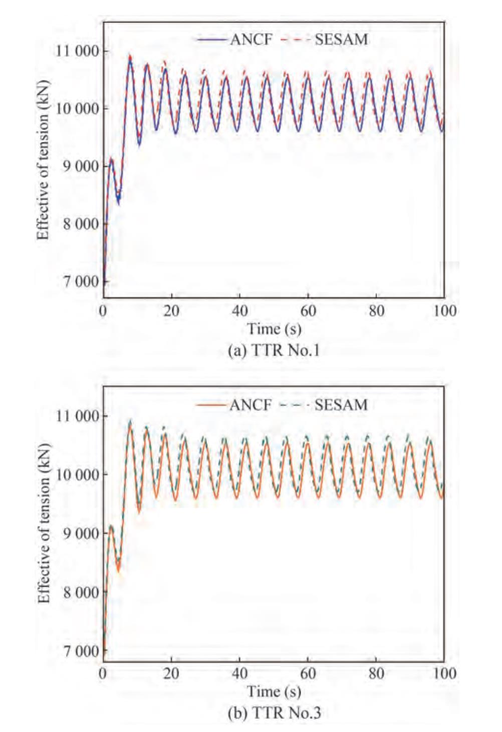 Figure 7 Time domain result of tension at the top node of the TTRTable 6 Effective tension at the top node of the tendon/TTR system for ANCF and SESAM
Method ANCF (MN) SESAM (MN) Error (%) TD1 Max 25.06 25.21 -0.590 Min 19.66 19.69 -0.155 Mean 22.66 22.77 -0.485 TD3 Max 25.05 24.96 0.390 Min 19.65 19.42 1.153 Mean 22.66 22.50 0.682 TTR1 Max 10.845 10.939 -0.867 Min 6.928 6.958 -0.433 Mean 10.006 10.082 -0.760 TTR3 Max 10.845 10.939 -0.867 Min 6.928 6.958 -0.433 Mean 10.006 10.082 -0.760 To study the influence of the amplitude of the top node forced motion, the sinusoidal excitation amplitudes are set as 2, 5, 10, and 20 m; the period is 12.0 s; and the motion is in the x-direction. The calculation time is set to 120 s, and the time step is 10-2 s. Figure 8 shows the effective tension at the top node of the tendon/TTR system. The maximum tension at the top node of the tendons/TTRs increases with the amplitude in the same period. Figure 8(a) indicates that the maximum tension of the tendon increases from 21.17 MN to 65.96 MN when the TLP amplitude increases from 2 to 20 m. Figure 8(b) implies that the maximum tension of the TTR increases from 8.674 to 44.686 MN when the TLP amplitude increases from 2 to 20 m. This finding proves that the tension variation of the TTR is larger than that of the tendon.
 Figure 8 Time domain result of the top node of the tendon/TTR with different TLP amplitudes
The reaction curve in each cycle presents a relatively regular sine pattern when the excitation amplitude changes from 2 to 20 m. If the motion period is consistent, then the corresponding velocity and acceleration of the riser will increase with the excitation amplitude. The riser will present the hysteresis phenomenon in motion because of its slender structural feature, which will further influence the variation of the effective tension of the top node.
The influence of the excitation period of the top node forced motion was also investigated. The sinusoidal excitation periods are set as 12, 16, 20, and 24 s. The amplitude is kept at 5 m, and the motion is still in the x-direction. Figure 9 shows the time domain and the maximum tension at the top node of the tendon/TTR system under different periods and indicates that the overall tension amplitude decreases with the excitation period. Figure 9(a) shows that when the TLP periods increase from 12 to 24 s, the maximum tension of the tendon decreases from 25.06 MN to 20.95 MN, which shows that TLP periods decrease two times and the maximum tension decreases 1.19 times. The oscillation amplitude of tension on the tendon decreases with the increase in the TLP periods. As shown in Figure 9(b), the maximum tension of the TTR decreases from 10.845 to 10.109 MN as the TLP amplitude periods increase from 12 to 24 s, indicating that the maximum tension decreases 1.07 times. The oscillation amplitude of tension on the TTR increases as the period increases, indicating that the variation in tension at the top node of the tendon is more significant than that in the TTR. Table 7 shows the tension results at the top node of the tendon/TTR system for different TLP amplitudes and periods. The maximum tension of the tendon and TTR is 6.596 and 44.686 MN, respectively, corresponding to an amplitude of 20 m and a TLP period of 12 s. When the amplitude is equal to 5 m and the TLP period is 12 s, the tension of the tendon and the TTR is minimum and equal to 19.66 and 6.928 MN, respectively.
 Figure 9 Time domain result of the top node of the tendon/TTR with different TLP periodsTable 7 Effective tension at the top node of the tendon/TTR system from different TLP amplitudes and periods
Items Case Max tension (MN) Min tension (MN) Tendon
T = 12 s2 m 21.17 19.67 5 m 25.06 19.66 10 m 35.36 19.68 20 m 65.96 19.69 Tendon
A = 5 m12 s 25.06 19.66 16 s 23.09 19.66 20 s 21.48 19.67 24 s 20.95 19.67 TTR
T = 12 s2 m 8.674 6.952 5 m 10.845 6.929 10 m 18.683 6.940 20 m 44.686 6.958 TTR
A = 5 m12 s 10.845 6.929 16 s 10.691 6.939 20 s 10.586 6.946 24 s 10.109 6.949 Figure 10 shows the motion trajectories of the tendon/TTR No.1 at different time points with A = 5 m and T = 12 s. From Figure 10, in the same period and amplitude of the forced harmonic motion, the motion of the TTR is more intense than that of the tendon because the TTR is less stiff than the tendon.
 Figure 10 Configuration of tendon No.1 and TTR No.1 at different times
To study the influence of the TLP motion and current force acting on the tendon/TTR system, the current with the velocity of 0.83 m/s is applied at the surface in the x-direction while the TLP motion conditions are kept the same as mentioned previously. The calculation time is set to 120 s, and the time step is set to 10-2 s. Figure 11 shows the tension at the top node of the tendons/TTRs in the time domain for two cases: only TLP motion and under TLP motion+current. The maximum tension of the tendon in Figure 11(a) is 25.06 MN in the case of TLP motion only and 26.09 MN in the case of TLP motion+current. The maximum tension increased by 1.03 MN, which is 4.09%. Figure 11(b) shows that the maximum tension of TTR is 10.845 MN in the case of TLP motion only and 11.757 MN in the case of TLP motion+current. The maximum tension is increased by 0.912 MN, namely, 8.41%. This finding demonstrates that the change in tension at the node at the top of the TTR is greater than that of the tendon and that the tension at the top node experiences both the TLP and the current load.
 Figure 11 Time domain result of tension at the top node of the tendon/TTR for ANCF in the case of TLP motion+current
Figure 12 shows the tension at the top node of the tendons/TTRs from ANCF and SESAM in the case of TLP motion+current. The tensions at the top node of the tendons/TTRs in both ANCF and SESAM are very close. The max/min tension at the top node of the tendons/TTRs for different environmental conditions are shown in Table 8. The maximum tension error is 1.031% at the top node of the TTR. Thus, the ANCF model can be applied to investigate the tension at the top node of the tendons/TTRs and can obtain accurate results with few elements.
 Figure 12 Time domain result of tension at the top node of the tendon/TTR from ANCF and SESAM in the case of TLP motion+ currentTable 8 Max/min tension at the top node of the tendon/TTR from ANCF and SESAM in the case of TLP motion+current
Items Max tension (MN) Min tension (MN) ANCF SESAM Error (%) ANCF SESAM Error (%) TD 26.09 26.44 1.339 19.66 19.71 0.263 TTR 11.756 12.086 2.730 6.931 7.003 1.031 4.3 Calculation and analysis under regular wave conditions
In dynamic analysis, the regular wave is 180°. The wave period is set to 21.17 and 9.77 s, and the wave amplitude is 1.67 m. The time for the dynamic analysis is set to 800 s, and the time step is 10-2 s.
Figure 13 compares the six-degrees-of-freedom motions of the TLP in the time domain for the experiment, ANCF, and SESAM in the case of T = 21.17 s. The maximum displacement of TLP in x-, y-, and z-directions for the experiment is 0.636, 0.066, and 0.013 m, respectively. The corresponding ones for ANCF are 0.473, 0.025, and 0.034 m, respectively, and those for SESAM are 0.581, 0.023, and 0.035 m, respectively.
 Figure 13 Motions of the TLP for ANCF, experiment, and SESAM in the case of regular wave (T = 21.17 s)
The maximum rotation of TLP in roll, pitch, and yaw for ANCF, experiment, and SESAM is small (maximum rotation is 0.032° in pitch). In general, the six-degree-of-freedom motions of TLP in ANCF, experiment, and SESAM have a similar trend.
Figure 14 compares the effective tension at the top node of tendons No.1, No.2, No.3, and No.4 in the time domain for ANCF, experiment, and SESAM. Figure 14 shows small oscillations of four tendons in the experiment, from 18.91 MN to 20.62 MN, while those in ANCF and SESAM are from 18.39 MN to 21.34 MN and from 17.27 MN to 21.50 MN, respectively. The maximum errors of the tension are 4.686% and 1.532%, respectively, when compared with the experiment and SESAM. The minimum ones are 2.828% and 0.559%, respectively.
 Figure 14 Effective tension at the top node of tendons No. 1–4 for ANCF, experiment, and SESAM in the case of regular wave (T = 21.17 s)
Figure 15 compares the effective tension at the top node of TTRs No.1, No.2, No.3, and No.4 in the time domain for ANCF, experiment, and SESAM. This figure shows that the amplitude of tension variation of four TTR in the experiment is minimal, ranging only from 6.833 MN to 6.896 MN, while the amplitude of tension variation of four TTR in ANCF and SESAM is from 6.126 MN to 8.264 MN and from 6.579 MN to 8.388 MN, respectively. The maximum tension error between ANCF and the experiment and SESAM is 16.568% and 1.490%, respectively, while the minimum tension error between ANCF and the experiment and SESAM is 16.446% and 1.163%, respectively. This result occurred because the upper end of the TTR is connected to the TLP by the spring system to measure the stiffness during the experiment, thus resulting in a smaller oscillation amplitude of the tension. In the ANCF model and SESAM, the upper end of the TTR is fixed with TLP, thus making the oscillation amplitude of the tension larger. Table 9 compares the maximum tension at the top node of the tendons/TTRs and the error values in the case of T = 21.17 s.
 Figure 15 Effective tension at the top node of TTR No. 1–No. 4 for ANCF, experiment, and SESAM in the case of regular wave (T = 21.17 s)Table 9 Comparison of the maximum tension at the top node of the tendons/TTRs for ANCF, experiment, and SESAM in the case of regular wave (T = 21.17 s)
Items Number ANCF
(MN)Experiment
(MN)Error
(%)SESAM
(MN)Error
(%)TD 1 21.21 20.35 4.055 21.54 1.532 2 21.22 20.62 2.828 21.50 1.302 3 21.34 20.34 4.686 21.46 0.559 4 21.33 20.56 3.610 21.46 0.606 TTR 1 8.246 6.886 16.493 8.343 1.163 2 8.245 6.889 16.446 8.343 1.175 3 8.264 6.896 16.554 8.388 1.478 4 8.263 6.894 16.568 8.388 1.490 Figure 16 shows the tension at the top node of tendon No.1 and TTR No.1 in the experiment, ANCF, and SESAM in the case of T = 9.77 s. From Figure 16(a), the maximum tension error on the tendon for ANCF and SESAM is 0.555%. The maximum tension on tendon No. 1 for the ANCF method in the case of T = 9.77 s is 21.37 MN, which increases by 0.16 MN compared with that in the case of T = 21.17 s. As can be seen from Figure 16(b), the maximum tension error of tension on the TTR for ANCF and SESAM is 0.236%, while it is approximately equal to 20% for ANCF and the experiment. In addition, the maximum tension on TTR No. 1 in the case of T = 9.77 s is 8.282 MN, which increases by 0.036 MN compared with that in the case of T = 21.17 s. This finding indicates that when the amplitude wave is constant and the impact direction is 180° on the TLP, the maximum tension of the tendon and TTR increases as the wave period decreases.
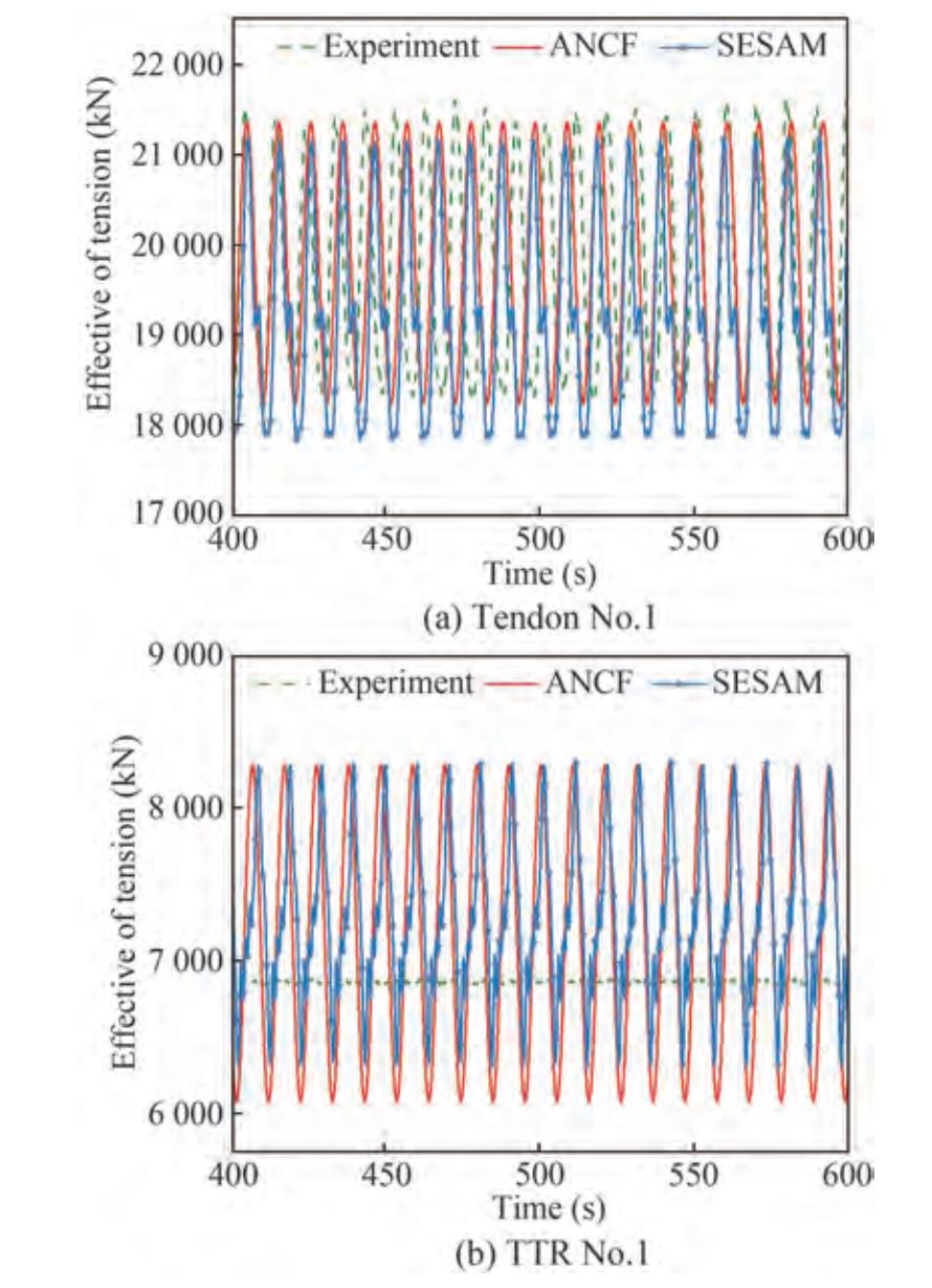 Figure 16 Effective tension at the top node of tendon No.1 and TTR No.1 for ANCF, experiment, and SESAM in the case of T = 9.77 s
Figure 17 shows the movement of the tendon/TTR No.1 at different time intervals for one period of waves.
 Figure 17 Configuration of tendon No.1 and TTR No.1 at different times
Consequently, the ANCF method can be applied to accurately simulate the motion of a TLP tendon/TTR coupled system with fewer elements.
5 Conclusion
In this study, the dynamics of the tendon/TTR system of a TLP are investigated. The numerical model of TLP tendons and TTRs is established based on the ANCF. The model is applied to study the static and dynamic characteristics of a TLP/tendon/TTR system. The calculation results of the ANCF model are compared with the results of an experiment and SESAM. The following conclusions are drawn:
1) A comparison of the results of ANCF with those of SESAM and the experiment shows that the tension at the top node of tendons/TTRs in the numerical simulation is in good agreement. Thus, the ANCF method in this study is reasonable and accurate for calculating multibody structure despite a lower element number.
2) The motion of the TTR is more intense than that of the tendon because the TTR is less stiff than the tendon. The tension occurs mainly on tendons. The tension of tendons/TTRs tends to increase with the increase in the TLP amplitude, the decrease in the TLP period, or the simultaneous action of the floating body and current.
Open Access This article is licensed under a Creative Commons Attribution 4.0 International License, which permits use, sharing, adaptation, distribution and reproduction in any medium or format, as long as you give appropriate credit to the original author(s) and thesource, provide a link to the Creative Commons licence, and indicateif changes were made. The images or other third party material in thisarticle are included in the article's Creative Commons licence, unlessindicated otherwise in a credit line to the material. If material is notincluded in the article's Creative Commons licence and your intendeduse is not permitted by statutory regulation or exceeds the permitteduse, you will need to obtain permission directly from the copyrightholder. To view a copy of this licence, visit http://creativecommons.org/licenses/by/4.0/. -
Figure 1 Layout of the experiment tendon/TTR of a TLP model system
Figure 2 Experiment model of the tendons and TTRs
Figure 3 Three-dimensional solid beam element model
Figure 4 Schematic model of TLP with tendon/TTR system
Figure 5 Effective tension of the tendons/TTRs under static condition
Figure 6 Time domain result of tension at the top node of the tendon
Figure 7 Time domain result of tension at the top node of the TTR
Figure 8 Time domain result of the top node of the tendon/TTR with different TLP amplitudes
Figure 9 Time domain result of the top node of the tendon/TTR with different TLP periods
Figure 10 Configuration of tendon No.1 and TTR No.1 at different times
Figure 11 Time domain result of tension at the top node of the tendon/TTR for ANCF in the case of TLP motion+current
Figure 12 Time domain result of tension at the top node of the tendon/TTR from ANCF and SESAM in the case of TLP motion+ current
Figure 13 Motions of the TLP for ANCF, experiment, and SESAM in the case of regular wave (T = 21.17 s)
Figure 14 Effective tension at the top node of tendons No. 1–4 for ANCF, experiment, and SESAM in the case of regular wave (T = 21.17 s)
Figure 15 Effective tension at the top node of TTR No. 1–No. 4 for ANCF, experiment, and SESAM in the case of regular wave (T = 21.17 s)
Figure 16 Effective tension at the top node of tendon No.1 and TTR No.1 for ANCF, experiment, and SESAM in the case of T = 9.77 s
Figure 17 Configuration of tendon No.1 and TTR No.1 at different times
Table 1 Main scale parameters and attributes of the TLP model
Parameter Full scale Model scale Depth of water (m) 663 10 Draft design (m) 21 0.317 Diameter of the column (m) 19 0.287 Spacing of the column center (m) 59 0.890 Freeboard of the column (m) 11.5 0.173 Column height (m) 32.5 0.490 Width of the pontoon (m) 11 0.166 Height of the pontoon (m) 8 0.121 Floating tank length (m) 40 0.603 Displacement (reign) (MT) 39 249 0.135 Center of gravity Xg (m) 0.0 0.000 Center of gravity Yg (m) 0.0 0.000 Center of gravity Zg (m) 29.01 0.438 Inertial radius Rxx (m) 31.59 0.476 Inertial radius Ryy (m) 31.59 0.476 Inertia radius Rzz (m) 31.44 0.473 Table 2 Physical parameters of each tendon and TTR
Items Outer diameter
(mm)Dry weight
(kg/m)Axial stiffness EA
(N)Total length
(m)Pretension
(MT)Real TD 812.8 578.63 1.474E10 644 1 000 TTR 365.1 242 4.00E9 679 139.8 Model TD 0.017 0.257 9.78E4 9.71 65.4 TTR 0.012 0.269 7.38E4 10.24 23.3 Table 3 Upper and lower positions of each tendon and TTR
Items Upper point Lower point x (m) y (m) z (m) X (m) Y (m) Z (m) Real TD1 36.218 36.218 2.00 36.218 36.218 -663 TD2 36.218 -36.218 2.00 36.218 -36.218 -663 TD3 -36.218 -36.218 2.00 -36.218 -36.218 -663 TD4 -36.218 36.218 2.00 -36.218 36.218 -663 TTR1 6.00 11.75 37.00 6.00 11.75 -663 TTR2 6.00 -11.75 37.00 6.00 -11.75 -663 TTR3 -6.00 -11.75 37.00 -6.00 -11.75 -663 TTR4 -6.00 11.75 37.00 -6.00 11.75 -663 Model TD1 0.546 0.546 0.030 0.546 0.546 -10 TD2 0.546 -0.546 0.030 0.546 -0.546 -10 TD3 -0.546 -0.546 0.030 -0.546 -0.546 -10 TD4 -0.546 0.546 0.030 -0.546 0.546 -10 TTR1 0.091 0.177 0.558 0.091 0.177 -10 TTR2 0.091 -0.177 0.558 0.091 -0.177 -10 TTR3 -0.091 -0.177 0.558 -0.091 -0.177 -10 TTR4 -0.091 0.177 0.558 -0.091 0.177 -10 Table 4 Test cases
Case Test period (s) Real period (s) 1 0.67 5.46 2 0.78 6.35 3 0.85 6.92 4 0.97 7.90 5 1.10 8.96 6 1.20 9.77 7 1.55 12.62 8 1.90 15.47 9 2.25 18.32 10 2.39 19.46 11 2.6 21.17 Table 5 Effective tension of tendons and TTRs for ANCF and SESAM
Method ANCF (kN) SESAM (kN) Error (%) TD Max 19 686.857 19 686.857 1.016×10⁻⁶ Min 19 099.377 19 095.909 0.018 Mean 19 396.887 19 393.638 0.017 TTR Max 6 957.984 6 957.984 5.749×10⁻⁶ Min 2 518.840 2 419.091 3.960 Mean 4 759.638 4 664.320 2.002 Table 6 Effective tension at the top node of the tendon/TTR system for ANCF and SESAM
Method ANCF (MN) SESAM (MN) Error (%) TD1 Max 25.06 25.21 -0.590 Min 19.66 19.69 -0.155 Mean 22.66 22.77 -0.485 TD3 Max 25.05 24.96 0.390 Min 19.65 19.42 1.153 Mean 22.66 22.50 0.682 TTR1 Max 10.845 10.939 -0.867 Min 6.928 6.958 -0.433 Mean 10.006 10.082 -0.760 TTR3 Max 10.845 10.939 -0.867 Min 6.928 6.958 -0.433 Mean 10.006 10.082 -0.760 Table 7 Effective tension at the top node of the tendon/TTR system from different TLP amplitudes and periods
Items Case Max tension (MN) Min tension (MN) Tendon
T = 12 s2 m 21.17 19.67 5 m 25.06 19.66 10 m 35.36 19.68 20 m 65.96 19.69 Tendon
A = 5 m12 s 25.06 19.66 16 s 23.09 19.66 20 s 21.48 19.67 24 s 20.95 19.67 TTR
T = 12 s2 m 8.674 6.952 5 m 10.845 6.929 10 m 18.683 6.940 20 m 44.686 6.958 TTR
A = 5 m12 s 10.845 6.929 16 s 10.691 6.939 20 s 10.586 6.946 24 s 10.109 6.949 Table 8 Max/min tension at the top node of the tendon/TTR from ANCF and SESAM in the case of TLP motion+current
Items Max tension (MN) Min tension (MN) ANCF SESAM Error (%) ANCF SESAM Error (%) TD 26.09 26.44 1.339 19.66 19.71 0.263 TTR 11.756 12.086 2.730 6.931 7.003 1.031 Table 9 Comparison of the maximum tension at the top node of the tendons/TTRs for ANCF, experiment, and SESAM in the case of regular wave (T = 21.17 s)
Items Number ANCF
(MN)Experiment
(MN)Error
(%)SESAM
(MN)Error
(%)TD 1 21.21 20.35 4.055 21.54 1.532 2 21.22 20.62 2.828 21.50 1.302 3 21.34 20.34 4.686 21.46 0.559 4 21.33 20.56 3.610 21.46 0.606 TTR 1 8.246 6.886 16.493 8.343 1.163 2 8.245 6.889 16.446 8.343 1.175 3 8.264 6.896 16.554 8.388 1.478 4 8.263 6.894 16.568 8.388 1.490 -
Bulín R, Hajžman M, Polach P (2017) Nonlinear dynamics of a cablepulley system using the absolute nodal coordinate formulation. Mechanics Research Communications 82: 21-28. https://doi.org/10.1016/j.mechrescom.2017.01.001 Ceng X, Shen X, Wu J (2007) Govering equations and numerical solutions of tension leg platform with finite amplitude motion. Applied Mathematics and Mechanics 28(1): 37-49. https://doi.org/10.1007/s10483-007-0105-1 Čepon G, Boltežar M (2009) Dynamics of a belt-drive system using a linear complementarity problem for the belt-pulley contact description. Journal of Sound & Vibration 319(3-5): 1019-1035. https://doi.org/10.1016/j.jsv.2008.07.005 Chandrasekaran S, Jain AK (2002) Triangular configuration tension leg platform behaviour under random sea wave loads. Ocean Engineering 29(15): 1895-1928. https://doi.org/10.1016/S0029-8018(01)00111-1 Chandrasekaran S, Nagavinothini R (2018) Tether analyses of offshore triceratops under wind, wave and current. Marine Systems Ocean Technology 13(1): 34-42. https://doi.org/10.1007/s40868-018-0043-9 Datta N (2017) Vortex-induced vibration of a tension leg platform tendon: multi-mode limit cycle oscillations. Journal of Marine Science and Application 16(4): 7. https://doi.org/10.1007/s11804-017-1440-8 Gerstmayr J, Shabana AA (2006) Analysis of thin beams and cables using the absolute nodal co-ordinate formulation. Nonlinear Dynamics 45(1-2): 109-130. https://doi.org/10.1007/s11071-006-1856-1 Gu J, Yang J, Lv H (2012) Studies of TLP dynamic response under wind, waves and current. China Ocean Engineering 26(3): 363-378. https://doi.org/10.1007/s13344-012-0028-y Jameel M, Oyejobi DO, Siddiqui NA, Ramli Sulong NH (2017) Nonlinear dynamic response of tension leg platform under environmental loads. KSCE Journal of Civil Engineering 21(3): 1022-1030. https://doi.org/10.1007/s12205-016-1240-8 Jia H (2012) Numerical and experimental studies on motions and mooring characteristics of a tension leg platform in the water depth of 1500m. Shanghai Jiao Tong University Lim FK, Hatton S (1991) Design considerations for TLP risers in harsh environment. International Society of Offshore and Polar Engineers Liu Cheng, Tian Qiang, Yan Dong, Hu Haiyan (2013) Dynamic analysis of membrane systems undergoing overall motions, large deformations and wrinkles via thin shell elements of ANCF. Computer Methods in Applied Mechanics Engineering Structures 258: 81-95. https://doi.org/10.1016/j.cma.2013.02.006 Ma G, Sun L (2014) Static analysis of the mooring line under large deformation by utilizing the global coordinate method. Journal of Harbin Engineering University (6): 674-678. https://doi.org/10.3969/j.issn.1006-7043.201306006 Ma L, Wei C, Ma C, Zhao Y (2020) Modeling and verification of a RANCF fluid element based on cubic rational Bezier volume. Journal of Computational Nonlinear Dynamics 15(4): 041005. https://doi.org/10.1115/1.4046206 Malayjerdi E, Ahmadi A, Tabeshpour MR (2016) Dynamic Analysis of TLP in intact and damaged tendon conditions. In The 18th Marine Industries Conference (MIC2016) Mansour AM, Huang EW, Phadke AC, Zhang SS (2006) Tension leg platform survivability analysis. In International Conference on Offshore Mechanics & Arctic Engineering 477-483 Muehlner E (2017) Tension Leg Platform (TLP). John Wiley & Sons, Ltd. Obrezkov L, Eliasson P, Harish AB, Matikainen MK (2021) Usability of finite elements based on the absolute nodal coordinate formulation for deformation analysis of the Achilles tendon. International Journal of Non-Linear Mechanics 129. https://doi.org/10.1016/j.ijnonlinmec.2020.103662 Obrezkov LP, Matikainen MK, Harish AB (2020) A finite element for soft tissue deformation based on the absolute nodal coordinate formulation. Acta Mechanica 231(4): 1519-1538. https://doi.org/10.1007/s00707-019-02607-4 Shabana AA (1997) Definition of the slopes and the finite element absolute nodal coordinate formulation. Multibody System Dynamics 1(3): 339-348. https://doi.org/10.1023/A:1009740800463 Shabana AA (2015) ANCF tire assembly model for multibody system applications. Journal of Computational and Nonlinear Dynamics 10(2): 024504. https://doi.org/10.1115/1.4028479 Tur M, Garcia E, Baeza L (2014) A 3D absolute nodal coordinate finite element model to compute the initial configuration of a railway catenary. Engineering Structures 71(1): 234-243. https://doi.org/10.1016/j.engstruct.2014.04.015 Wang L, Currao G, Han F (2017) An immersed boundary method for fluid-structure interaction with compressible multiphase flows. Journal of Computational Physics 346: 131-151. https://doi.org/10.1016/j.jcp.2017.06.008 Yan GW, Xu F, Zhu H (2009a) Dynamic response analysis of TLP's tendon in current loads. https://doi.org/10.1007/978-90-481-2822-8_62 Yan GW, XU F, Zhu H, OU JP (2009b) Dynamic response analysis of TLP's tendon in wave and current. China Ocean Yang CK, Kim MH (2010) Transient effects of tendon disconnection of a TLP by hull-tendon-riser coupled dynamic analysis. Ocean Engineering 37(8-9): 667-677. https://doi.org/10.1016/j.oceaneng.2010.01.005 Zhang C (2020) Research on characteristics of vortex-induced vibration for deepwater riser considering dynamic boundary coupling effect. Harbin Engineering University 147-149 Zhang C, Kang Z, Ma G, Xu X (2019) Mechanical modeling of deepwater flexible structures with large deformation based on absolute nodal coordinate formulation. Journal of Marine Science and Technology 24 (12): 1241-1255. https://doi.org/10.1007/s00773-018-00621-0 Zhang C, Lu L, Cao QY, Cheng L, Tang GQ (2022) Nonlinear motion regimes and phase dynamics of a free standing hybrid riser system subjected to ocean current and vessel motion. Ocean Engineering 252: 111197 Zhang H, Smith D (2017) Interference of top tensioned risers for tension leg platforms. Offshore and Arctic Engineering Volume 5B. https://doi.org/10.1115/OMAE2017-61334 Zhang Y, Wei C, Zhao Y, Tan C, Liu YJ (2018) Adaptive ANCF method and its application in planar flexible cables. Acta Mechanica Sinica 34(1): 199-213. DOI: 10.1007/s10409-017-0721-4
