1   Introduction

Critical buckling loads can be calculated for tubular members using empirical equations. These equations are presented by design codes such as API RP-2A WSD and API RP 2A-LRFD (Recommended Practice for Planning, Designing, and Constructing Fixed Offshore Platforms), ISO 19902 and NORSOK N-004 to achieve load and resistance design factors. All these codes have been checked in order to assure that design loads do not meet critical buckling loads in normal and extreme operational conditions. Also, both global elastic buckling and inelastic buckling are covered by design codes that prevent local buckling in walls of tubular members by decreasing the loads. Even to ensure that applied loads do not exceed the critical buckling loads in normal operations, these codes explain the structural configuration of members.

Some members compress higher than their buckling limit under extreme load conditions such as ductility level earthquake (DLE) and the results of this case on the behavior of the structure also need to be examined. It is possible that the structures are designed in such a way that local buckling occurs in some members under extreme loads. Subsequently, in the process of analysis, it is checked that the level of structural failure remains within acceptable limits. In this analysis, the actual response of the structure is obtained. For this purpose, load and capacity factors are equal to 1. It is important that the local buckling of members and their post-buckling behavior are detected, correctly. So that the load transfer to adjacent elements is not underestimated. Nonlinear finite element models with 1-D beam elements are usually used to analyze the collapse of jacket structures. However, the beam elements do not consider the local buckling response and local deformation of the walls of members. Local buckling often does not occur in members with a low ratio of diameter-to-thickness (D/t). As the diameter-to-thickness ratio increases, the local buckling event leads to a further drop in post-buckling capacity in comparison with the value predicted by using the beam element. Also, models with beam elements cannot directly consider radial and circumferential imperfections due to fabrication tolerances which reduce load-carrying capacity. When solid elements are used to model thin-walled tubular members, the model elements can consider global and local buckling at solid walls simultaneously. The following is an overview of the research that has been conducted to investigate the buckling of the tubular members.

Xia and Hoogenboom (2011) checked the buckling of the frame members when the buckling length was set manually. Based on their estimation, 5% to 10% of the man-hours in structural analysis of removal projects is spent on checking and correcting buckling lengths. Using another method is available that does not require determining buckling lengths. In the study, the NORSOK standard for tubular steel frame structures was used to derive this method. They concluded that this method can be successfully applied. Karamanos and Tassoulas (1996) derived curves concerning the capacity of tubular members using a nonlinear FE technique under the combination of external pressure and bending. Yasseri et al. (2006) studied the global and local buckling of and their interaction for tubular members under concentrated force and moment. They classified the compressive members based on the diameter-to-thickness ratio (D/t) and the ratio of length-to-gyration radius (L/r). They proposed the suggested API curve of elastic and non-elastic buckling based on the slenderness. They also studied the effects of the imperfection of compressive members. The modified properties of steel material which can be used for beam elements to achieve the same response as shell elements were also presented in that report. Wang and Shenoi (2019) performed both numerical and experimental studies to investigate the effects of pitting damage on the structural performance and buckling behavior of tubular members. Their paper was selected by the author as one of the verification experimental references in this paper. Marshall (1992) presented some useful buckling curves of columns and provides good insight into the buckling behavior of tubular members under axial load for both pinned and fixed supports. Talaeitaba et al. (2015) used solid elements in ABAQUS FE for modeling columns with different circular cross-sections. They verified the models in agreement with experimental data. The authors reproduced some of the presented curves in their paper. Sadowski and Rotter (2013) investigated the structural behavior of tubular columns under the buckling phenomenon considering Shell elements. USFOS Verification Manual (2010) designed an experimental program to compare the behavior of un-grouted and grouted tubular columns subjected to compressive loading. The information about tests was also described in two other reports by offshore design (2000) and Haukaas and Yang (2000). The authors of this paper focused on an un-grouted circular hollow section with a given external diameter, wall thickness, and length. This experimental program was adopted by the authors as second verification experimental reference in this paper. Bardi and Kyriakieds (2006) and Bardi et al. (2006) studied the plastic buckling range of thick cylindrical shells. They focused on circular stainless-steel tubes in both experimental and analytical phases. Hu et al. (1993) investigated imperfections and their influence on the structural behavior of unstiffened, fabricated, tubular beam-columns. A comparison of experimental, analytical, and finite element analysis results has been discussed in this study. However, the nature and magnitude of imperfections in fabricated tubular members greatly differ from those found in seamless circular hollow sections. Buchanan et al. (2018) undertook a comprehensive experimental program to study the buckling behavior of stainless-steel circular hollow sections columns. The experimental plan of their research covered a wide range of diameters, thicknesses, lengths, and materials' mechanical and chemical properties. Their paper is the third verification experimental reference in this paper.

A sudden or gradual drop in post-buckling load capacity is created where the interaction between the global and local buckling is established which 2D beam elements cannot predict. In addition, radial and circumferential imperfections due to manufacturing deficiencies do not directly consider by beam elements (Karampour, 2018). These deficiencies can reduce load capacity significantly.

Modeling of thin-walled tubular members with solid elements can consider local and global buckling and their interaction simultaneously. Also due to the modeling of thickness in solid elements, the effects of stress concentration are simulated on the thickness of the member. Regarding the literature review and the authors' experiences in studying the buckling phenomenon, the effects of local buckling under compressive axial force do not properly investigate by shell elements without global bending moments. So, solid elements are selected to study the effects of five different parameters on compressive members in this paper. These five parameters include D/t, L/D, mesh size, mesh size ratio, and imperfections. In this study, after three levels of fundamental verification on modeling of buckling and post-buckling behavior of tubular members based on reliable experimental articles, the effects of five intended parameters on different parts of buckling and post-buckling behavior of such members have been investigated. All the main findings have been addressed in the paper. Consequently, it has been concluded that the mesh size along the length of a member is the most effective parameter in the occurrence of plastic local buckling. Moreover, it is shown that mesh ratio is the most effective parameter on the accuracy of elastic stiffness and post-buckling strength and the imperfection is significantly the most important factor regarding the proper estimation of the critical buckling load.

2   Finite element modeling

2.1   Range of parameters

Changes in the buckling and post-buckling behavior of tubular members are evaluated in this paper under the influence of each of the five desired parameters which include: diameter-to-thickness (D/t), length-to-diameter (L/D), number of mesh elements on cross-section, mesh size ratio (aspect ratio of mesh size on length to mesh size on the section) and imperfection. Two ratios of 30 and 80 for D/t and four ratios of 20, 30, 50, and 70 for L/D are chosen considering the typical dimensions of the braces of the Persian Gulf jacket platforms. Four values of 8, 16, 32, and 64 for the number of mesh elements on cross-section, three values of one-third, 1, and 3 for the mesh ratio, and three values of L/500, L/1000, and L/2000 for the imperfection are considered in this paper as the variable parameters. It should be noted that researchers typically use and propose the value of L/1000 (0.1% of the length of the member) as imperfections (Feng et al., 2004; Dhanens et al., 1993). In this paper, in addition to the imperfection L/1 000, half and twice this value have been checked to evaluate the proposed value of imperfection by references (Dhanens et al., 1993; Thai et al., 2015).

Each of the above categories is analyzed with separate finite element models using 3D solid elements. For each model, a distinct modal buckling analysis is performed and eigenvalues are calculated. The imperfection is assigned as a coefficient of the first buckling mode shape after the modal buckling analysis of each model (Thai et al., 2015). Totally 384 analyses were performed in this paper considering modal buckling analyses.

2.2   Analysis methodology

The static Riks analysis method has been used in ABAQUS software because the other analysis methods become unstable under a sudden reduction in stiffness due to buckling. In the Riks procedure, deformations and loads are considered simultaneously. This means that the magnitude of the load is taken as a variable and the arc length method, in static equilibrium in the load-displacement space, is used to obtain the solution. The load-deflection (Riks) analysis can be performed when concerned about geometric (Nlgeom) or material nonlinearity prior to buckling or unstable post-buckling response exist. Otherwise, in other cases, the typical linear or nonlinear static analysis may be stable. Despite all the benefits of Riks analysis, this method is much more complex than Newton Raphson's static general method (Abaqus documentation, 2012). So, the ABAQUS program is able to discover the post-buckling response of the model by reducing the applied load and solving the load-displacement equation (Priyadarsini et al., 2012).

All of the finite element models with or without imperfection are analyzed by this method. Then the buckling and post-buckling responses of all parameters are compared.

2.3   Material model

The assigned material for all the compressive members was Steel material with Young's modulus of 210 GPa, poisson ratio of 0.3 and yield stress of 360 MPa. Ramberg-Osgood material properties have been used to produce the stress-strain curve of material according to its yield stress and elastic modulus. Von Mises yield criterion was assumed. The narrowing test of the coupon bar under axial load is used to obtain true stresses (Ramberg and Osgood, 1943). The values of true stresses and logarithmic strains are calculated from the nominal experimental values using the following equations.

Initial geometric known as imperfections can be categorized into two main parts. First category is local imperfection such as ovalization in section of member and the second one is global imperfection such as out-of-straightness of member (Tao et al., 2007). The purpose of imperfection in this paper is initial global geometric defects which means eccentricity from longitudinal axis of tubular member caused by handling processes, manufacturing, and transporting (Hu et al., 1993). Therefore, no ovalization (local imperfection) has been assigned here.

2.4   Modeling elements

As mentioned before, 384 models using 3D solid elements have been performed assuming the outer diameter of 0.6 m. To the best of the authors' knowledge and referring to some references include Weaver and Dickenson (2003), Harding et al. (1982), Fajuyitan et al. (2018), Sadowski and Rotter (2013), and Silvestre (2008), the shell elements estimate of the buckling moment strength under uniform bending for cylinders members accurately. Hence, the use of solid continuum elements is uneconomical in terms of global bending. However, regarding to the literature, the effects of local buckling and its interaction with global buckling cannot be detected properly by shell elements under axial compression. Therefore, continuum 3D solid elements have been selected for the models of this paper with the abbreviation of C3D8R. It should be noted that all models have two mesh elements in thickness direction as seen in Figure 1.

Figure  1  Geometry and meshing configuration of a member with D/t=30, L/D=20, 32 number of elements on section, mesh ratio of 3

Download: Full-Size Img

In addition to 384 main models of paper, the authors also developed 192 models with one element and 192 models with four elements in thickness direction to confirm the effects of number mesh elements on thickness. After analyzing and comparing the results of these extra 384 models with main models it has been concluded that by applying one mesh element on thickness, local deformations or ovalizations during analysis in tube section cannot be evaluated correctly. So, many of the FE analysis diverged. For the dimensions of the tubular members assumed in this paper, regardless of the thickness of the member, at least two elements along the thickness seems to be required. Generally, for traditional tubular members in offshore structures with D/t ratio more than 25 and thickness value less than 4 cm, assigning more than two mesh elements in thickness will only increase the computational cost and no significant difference in the buckling and post-buckling strength of member will occur. The comparison curves of buckling and post-buckling behavior of models with different mesh number on thickness have been achieved but not presented here for the sake of brevity.

According to the results, only in some models with 2 elements in thickness, a bit more drop in post-buckling strength can be seen compared to the models with 4 elements. However, this can lead to a bit conservative estimation of the post-buckling capacity. So, all tubular members in this paper have been modeled with two elements in thickness direction.

2.5   Loading method and boundary conditions

The aim of this paper investigates the buckling behavior of tubular steel members under only axial compression. The purpose is to apply the axial compressive displacement to one end of the tubular members and to calculate the resultant reaction force on the other side, which is equal to the total load applied to the member. In this way, it is possible to achieve the load-displacement curve of the member that can illustrate the pre-buckling elastic behavior of the member, the loss of strength immediately after buckling and the post-buckling strength. Therefore, displacement-control approach was used instead of force-control. The maximum displacement of 0.5 meter has been applied to all members with different length and diameters. This amount of displacement is large enough for all members with various lengths and diameters to buckle. The MPC has been used for both edges and pinned support is selected as the boundary condition of both ends of the tube. No hydrostatic pressure was assumed in this paper. However, in the intended case study concerning modeling of jacket frame, hydrostatic pressure has been considered for all members.

3   Analytical equations for prediction of buckling

The comparison of the buckling prediction approaches of four different standards include API WSD, API LRFD, ISO, and NORSOK in detail have been described in this part. All four codes provide sets of formulations for each load type acting alone or in combination. ISO equation can be used with a high accuracy to predict the buckling of tubular sections (ISO 19902, 2007). All dimensional parameters have stress dimension.

Local buckling check in ISO and NORSOK is based on material as well as geometric properties of members whereas in API WSD and API LRFD it depends on only geometry parameters.

NORSOK code in the terms of local buckling strength has the similar approach to the ISO equation. There is only a slight difference in limitation. Contrary to ISO 19902 and NORSOK N-004, as it can be seen in Table 1, API WSD and LRFD codes, distinguish between elastic and inelastic buckling stresses.

According to the above local buckling equations, the maximum value of D/t ratio is limited to 120 in ISO and NORSOK codes, whereas the API increases the upper limit of D/t ratio to 300 which means that NORSOK is significantly more conservative.

The three API LRFD, ISO, and NORSOK codes have proposed same formulae form for column global buckling but have employed different coefficients. The overall column buckling formula in API WSD uses the AISC formulation, while API LRFD, ISO and NORSOK are LSD or LRFD based. The recommended equation of NORSOK code gives lower capacity than API LRFD and ISO. Unlike the other three standards, NORSOK code assumes that the platform is manned even during extreme environmental events, so in calculation of both local and overall buckling strength, NORSOK is more conservative.

The bending formulae of all four codes are the same but the API WSD has different coefficients. According to above equations, elastic section modulus (Z_e), plastic section modulus (Z_p), and yield strength (f_y) can be seen in formulae because LSD and LRFD approaches consider full plasticity and yielding in the section, whereas because of WSD methodology which limits the stress to a fraction of the yield, only the yield strength exist in API WSD equations. Also in evaluation of bending capacity NORSOK is more conservative than three others.

Reduction factors (C_m) corresponding to the cross-section directions are functions of the end moments, compressive stress and Euler buckling stresses.

Concerning the simultaneous effects of compression and bending on tubular members, the API WSD, ISO and NORSOK codes formulae have the same linear form with some partial differences, while API LRFD recommends a cosine form equation.

In Table 1,

4   Experimental results

In this paper, the verification of the effects of the desired parameters is made based on the results of three different series of validated experiments. The selected experiments are well adapted to the requirement of present paper. Also, these experiments have been published in reputable journals and frequently cited. Therefore, the authors reasonably decided to refer to these three experiments for verification of modellings. This part describes each of these experiments. Table 2 contains stress-strain data of steel material applied in FE modellings of all three verification experiments as derived from the related papers.

4.1   Experiment 1

Wang and Shenoi (2019) performed both numerical and experimental studies to investigate the effects of pitting damage on the structural performance and buckling behavior of tubular members. For this purpose, both intact and pitted members were tested. Experimental results of intact tubular members are addressed in this paper. The experimental setup in that paper is shown in Figure 2.

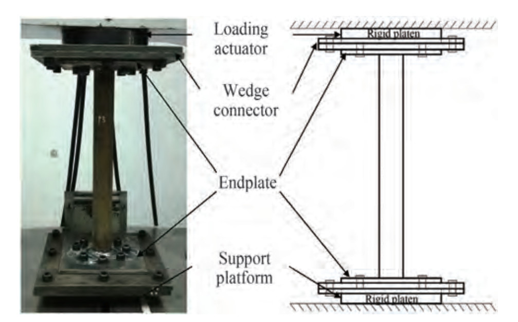Figure  2  Schematic diagram of test setup (Wang and Shenoi, 2019)

Download: Full-Size Img

The members had an external diameter of 54 mm, D/t ratio of 7.83, length of 460 mm, and were made from a seamless circular steel tube. Fixed-ended boundary condition was selected for both two ends. Two material tensile coupon tests and 14 member tests under compressive loads were included in the experimental program of their paper. Regarding to stress-strain curves of the two tensile specimen tests which is shown in Figure 3, the Young's modulus, E, yield stress, σ_y, and ultimate stress, σ_u of the selected steel material were 125 GPa, 311 MPa and 463 MPa, respectively.

Figure  3  Stress-strain curve of the two tensile specimen tests (Wang and Shenoi, 2019)

Download: Full-Size Img

The true stress and true strain data applied in numerical modeling of this section of paper and derived from the tensile tests can be seen in Figure 4.

Figure  4  Stress-strain relationship applied in numerical analysis (Wang and Shenoi, 2019)

Download: Full-Size Img

4.2   Experiment 2

This experimental program was designed to compare the behavior of un-grouted and grouted tubular columns subjected to compressive loading. The information about tests was described in three reports by offshore design (2000), Haukaas and Yang (2000), and USFOS verification manual (2010). This paper focuses on an un-grouted circular hollow section with external diameter of 160 mm, wall thickness of 4.5 mm, and length of 2 500 mm. Roller bearings located eccentrically to the pipe axis act as pinned-supports of both two ends. The schematic diagram and a view of test set-up and a buckled member have been shown in Figure 5. The circular hollow sections tested for this purpose were made of two types of high and low yield stress steel materials. The tests were carried out using high yield stress considered for FE analysis in this paper.

Figure  5  Schematic diagram of test setup-up and column in post-buckled condition (USFOS verification manual, 2010)

Download: Full-Size Img

4.3   Experiment 3

Buchanan et al. (2018) undertake a comprehensive experimental program to study the buckling behavior of stainless steel circular hollow sections columns. The experimental plan of their research covered both "stub column tests" and "flexural buckling tests". So, a wide range of diameters, thicknesses, lengths and materials mechanical and chemical properties were examined. Numerical modeling of this paper performs based on external diameter of 105.67 mm, thickness of 2.7 mm, and length of 3 083.0 mm with regard to reported results in their paper. Figure 6 illustrates set-up of flexural buckling tests. According to the test set-up pinned-end boundary condition in one direction as well as MPC constraint have been applied to both ends of tubular members. Both tensile and compressive coupon tests were carried out to extract mechanical properties of material. Young's modulus of 226.6 GPa, σ_0.2 of 250 MPa and σ_u of 614 MPa for tensile behavior and Young's modulus of 188.7 GPa, σ_0.2 of 276 MPa and σ_1.0 of 315 MPa for compressive behavior of material properties were imported in FE modeling. Ramberg-Osgood material properties have been used to produce the tensile and compressive stress-strain relationships from the tensile coupons and compressive stub column responses.

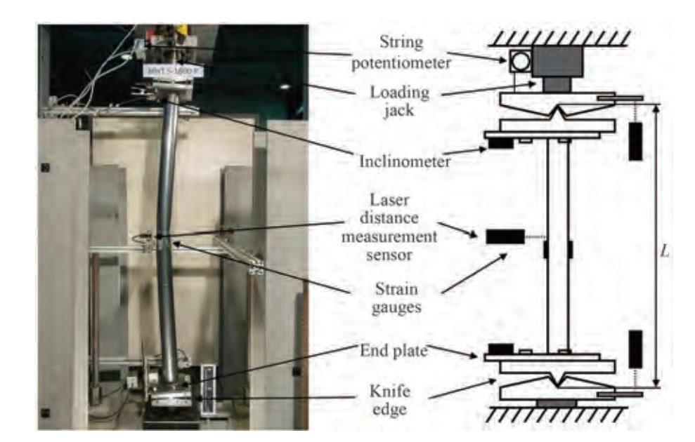Figure  6  Long column test set-up (Buchanan et al., 2018)

Download: Full-Size Img

5   Verification results

In this section results of verification of models against three main experimental data have been explained. Since changes in mesh size, mesh ratio and imperfection have been also applied in level of verification of models, the provided results can be adopted to achieve further accuracy in final conclusion of the paper.

5.1   Results of experiment 1

As the first step of verification, the bucked shape of the member obtained from FE analysis along with its experimental failure mode is illustrated in Figure 7, where close correlation may be observed. Also contours of stress values and plastic strain values are shown in Figure 7.

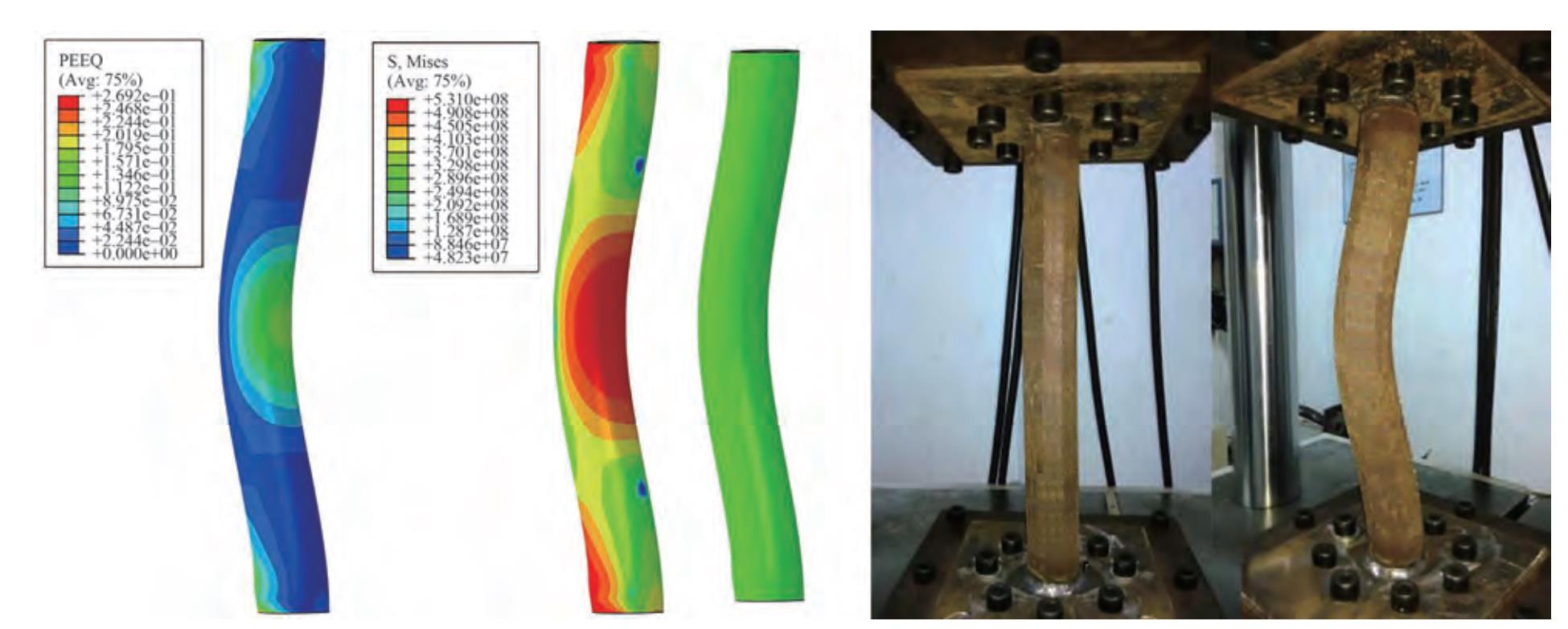Figure  7  Failure mode of typical experimental and numerical results, along with stress and plastic strain contours (Wang and Shenoi, 2019)

Download: Full-Size Img

The differences between FE models and experiments have been categorized in two phases including critical buckling loads and post-buckling strengths. In each category, one clustered column diagram has been drawn which represent error percentage changes versus mesh size ratio. Other diagrams representing the error percentage changes versus imperfection and number of mesh elements on section have been drawn for other two experiments and have been omitted for this experiment for the sake of brevity. Figure 8 and 9 clearly illustrate the effects of number of mesh elements on section, mesh size ratio, and imperfection on the accuracy of critical buckling load results and post-buckling strength, respectively. Two pushover curves of buckled and non-buckled (compressive yielding before buckling occurrence) models have been depicted in both diagrams.

Figure  8  The error changes of the results of critical buckling loads versus mesh size ratio-derived from models with different mesh number on section and different imperfections

Download: Full-Size Img

Figure  9  The error changes of the results of post-buckling strengths versus mesh size ratio-derived from models with different mesh number on section and different imperfections

Download: Full-Size Img

All of the errors above the red dashed line in the diagrams indicate that the desired model has not buckled with its mesh and imperfection conditions and compressive yielding has occurred.

Good agreement in predicting the initial stiffness can be observed in pushover curves which have been depicted in all diagrams for all three experimental verifications.

5.2   Results of experiment 2

The failure modes of the FE models show excellent agreement with those derived from the tests, as shown in Figure 10. The stress and equivalent plastic strain contours shown in Figure 10 confirm the presence of stress concentration in the middle of the member.

Figure  10  Experimental post-buckled condition along with deformed shape of FE analysis and stress and equivalent plastic strain contours (USFOS verification manual, 2010)

Download: Full-Size Img

As previous section, for this experiment two parameters of critical buckling load and post-buckling strength have been represented to indicate the differences between FE models and experiments in such a way that the error percentage of different models results have been presented as clustered column diagrams with respect to changes in imperfection values. These diagrams have been depicted in Figures 12 and 13. The pushover curves of two models have been randomly depicted in both diagrams.

Figure  11  Experimental and FE failure modes including stress and equivalent plastic strain contours (Buchanan et al., 2018)

Download: Full-Size Img

Figure  12  The error changes of the results of critical buckling loads versus imperfection-derived from models with different mesh number on section and different mesh size ratio

Download: Full-Size Img

Figure  13  The error changes of the results of post-buckling strengths versus imperfection-derived from models with different mesh number on section and different mesh size ratio

Download: Full-Size Img

As can be seen obviously, changing the mesh size ratio has almost no effect on the accuracy of critical buckling load and has no negligible effect on the accuracy of estimating the post-buckling strength, especially when the mesh size along the length of member is fine.

Imperfection value greatly affects the critical buckling load (Godat et al., 2012) but as is demonstrated later in this paper, changing the imperfection is almost ineffective in the post-buckling strength. Number of mesh elements on section is also an influential parameter either in critical buckling load or post-buckling strength in case of low number of mesh elements on section.

5.3   Results of experiment 3

There is an excellent agreement between experimental failure mode and FE result of this paper which are shown in Figure 11. The stress and equivalent plastic strain contours are seen in Figure 11 as well.

The differences between FE models and experimental results of this experiment have also been studied in two parts of accuracy of critical buckling load and accuracy of post-buckling strength. The clustered column diagrams which represent error percentage changes versus number of mesh elements on section have been shown in Figures 14 and 15. The pushover curves of two models have been randomly depicted in both diagrams. As clearly shown in the figures, imperfection has the greatest effect on critical buckling load, whereas the major effectiveness parameter on post-buckling strength is number of mesh elements on section. The same results have been concluded in the rest of this article.

Figure  14  The error changes of the results of critical buckling loads versus mesh number on section-derived from models with different imperfection and different mesh size ratio

Download: Full-Size Img

Figure  15  The error changes of the results of post-buckling strengths versus mesh number on section-derived from models with different imperfection and different mesh size ratio

Download: Full-Size Img

6   Results

In this part, some of the results of 384 models all with the same outer diameter of 0.6 m contain four different lengths, two different thicknesses, three different imperfections, four different number of mesh elements on section, and three different mesh size ratios on length relative to cross-section have been presented.

The differences between the critical buckling load obtained from the model results and its corresponding value calculated by the ISO equation for some models have been shown in Figure 16 to Figure 21. Also, the effect of each of the desired parameters on accuracy of critical buckling load, post-buckling strength and elastic stiffness results of tubular members with different D/t and L/r ratio can be seen in these figures. Desired parameters are mesh size ratio along the length to the cross-section, imperfection value and mesh numbers on tube section. These figures are selected in such a way all combinations of D/t and L/D ratios are covered.

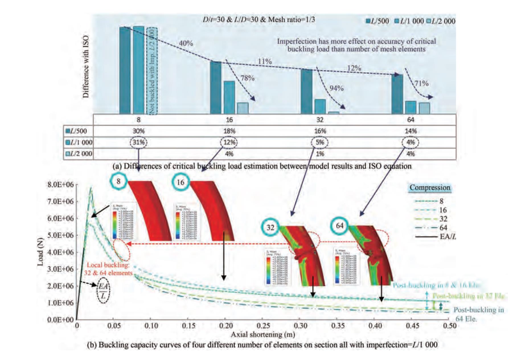Figure  16  The effect of number of tube section mesh elements on critical buckling load and post-buckling strength of a tubular member with D/t=30, L/D=30 and mesh ratio=1/3

Download: Full-Size Img

Figure  17  The effect of number of tube section mesh elements on critical buckling load and post-buckling strength of a tubular member with D/t=30, L/D=30 and Imp=L/500

Download: Full-Size Img

Figure  18  The effect of imperfection value on critical buckling load and post-buckling strength of a tubular member with D/t=80, L/D=30 and mesh ratio=1/3

Download: Full-Size Img

Figure  19  The effect of imperfection value on critical buckling load and post-buckling strength of a tubular member with D/t=80, L/D=20 and mesh number=64

Download: Full-Size Img

Figure  20  The effect of mesh ratio on critical buckling load and post-buckling strength of a tubular member with D/t=30, L/D=30 and mesh number=32

Download: Full-Size Img

Figure  21  The effect of mesh size ratio on critical buckling load and post-buckling strength of a tubular member with D/t=80, L/D=30 and imperfection=L/500

Download: Full-Size Img

According to the cluster column diagram of Figure 17 the mesh ratio parameter shows considerable effect on critical buckling load when the ratio of mesh size along the length to the section of a member is high. In other words, when the mesh size on length of member is sufficiently fine, decreasing the mesh ratio does not improve the accuracy of results.

It should be noted that the results of all 384 models and all the values of the differences between ISO equation and model results have been used to achieve the final conclusion of this paper. But for the sake of brevity, some of the figures are illustrated in this part and the rest are omitted.

Figure 16 clearly shows that the effect of imperfection on critical buckling load is higher than that of the number of mesh elements. However, it should be noted that imperfection has no effect on post-buckling strength while number of mesh element will certainly be effective. On the other hand, as can be found from Figure 17, the mesh ratio has more impact on accuracy of critical buckling load than number of mesh elements.

The phrase of "Not-Buckled" in some of the above cluster column diagrams means that due to insufficient imperfection or improper mesh size in member, compressive yield of material occurred earlier than the buckling under axial load. For this reason, some models have buckling non-occurrence conditions and therefore their results have not been considered in the study of the effects of five desire parameters.

Based on Figures 18 and 19, imperfection affects the accuracy of critical buckling load more than number of mesh elements. Also, it can be stated that mesh ratio does not have a significant effect on the accuracy of critical buckling load when it reduces from 1 to 1/3.

Another noteworthy point in Figures 18 and 19 is that imperfection only changes the critical buckling load value and does not affect post-buckling strength and elastic stiffness at all. Even the shapes of buckled members with different imperfections are quite similar.

Local buckling in the middle of the compressive member length known as kneeling occurs due to stress concentration in two side points of the tubular section wall. Contrary to popular belief, this phenomenon is formed by reducing D/t ratio. Since no global buckling is observed in tubular members with higher thickness due to the greater bending stiffness of them, which prevents the occurrence of overall deformation. Local buckling Occurrence can also affect the post-buckling strength. This fact can be clearly seen in the Figures 16, 17, 20 and 21.

A closer look at Figures 20 and 21 reveals that the lower mesh size ratio which means finer mesh along the length of the member is required to achieve more accurate estimation of the critical buckling load and post-buckling strength of the member. Since the mesh size ratio indicates the ratio of the mesh size along the length to the mesh size along the cross-section, so for a given member, the 1/3 mesh size ratio and 16 mesh elements on section results in a finer mesh along the length of member than the 3 mesh size ratio and 64 mesh elements on section.

As can be seen, kneeling phenomenon due to plastic buckling does not appear in members with coarse mesh along the length. So considering its effect on post-buckling behavior, proper mesh size along the length of compressive members seems necessary. It should be noted that coarse mesh size along the length also affects the critical buckling load and reduce its accuracy. This point is also well illustrated in Figures 20 and 21.

By increasing the D/t ratio the bending stiffness of tubular wall decreases with a power of 3 (Yasseri and Skinner, 2006). After occurrence of the buckling, the tubular member walls start to swing and ultimately the member bends. Local bending moments due to deformation of the tube wall quickly result a local plastic zone. Finally, the local buckling which reduces the capacity of member leads to global buckling. Increasing the L/r ratio concludes further plastic zone and fewer critical buckling load.

The enlarged plastic area causes a sudden collapse if the local buckling occurs in this state (Yasseri et al., 2006).

In general, the Figure 22 can represent the boundary of elastic and plastic buckling. Also, considering to all the results, both in the experimental validation section and in the FE modeling section, Figure 23 can be extracted as the effect area of each parameter on the buckling behavior of tubular members. Figure 24 exhibits the percentage of effect of each parameter including mesh size ratio, number of mesh elements on section, and imperfection on three main part of capacity curve of tubular members. These three main parts are accuracy of estimation of initial elastic stiffness, critical buckling load, and post-buckling strength.

Figure  22  The comparison of elastic buckling, plastic buckling, and compressive yielding based on L/r ratio

Download: Full-Size Img

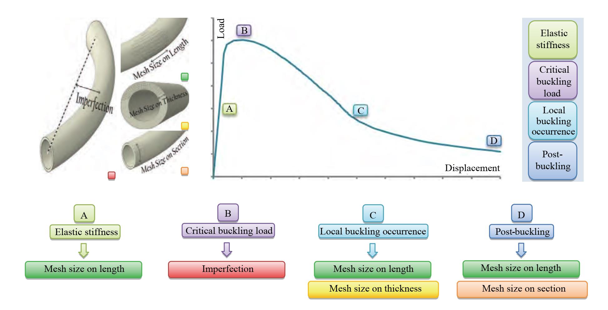Figure  23  The most affected part of each parameter on buckling capacity curve of tubular members

Download: Full-Size Img

Figure  24  The percentage of the effect of each parameter on the elastic stiffness, critical buckling load, and post-buckling strength of tubular members

Download: Full-Size Img

According to Figure 24 the mesh ratio (the mesh size along the length of member to the mesh size on the cross-section) is the most effective parameter on the accuracy of elastic stiffness and post-buckling strength. Similarly, as shown in Figure 24 the imperfection parameter is significantly the most important factor regarding to calculation of the critical buckling load (Godat et al., 2012).

7   Case study

A four-leg Resalat jacket platform of Persian Gulf was selected as case study to investigate the effect of desired parameters on buckling behavior of compressive members. The schematic geometry and dimensions of the jacket and model are shown in Figure 25. A 3-Dimensional model of one frame of jacket was provided. All of the joint cans and the principal details have been taken into account in FE modeling.

Figure  25  Schematic geometry of one row of Resalat jacket and FE model include global geometry of model, geometry of piles driven into legs, transition piece, tubular connections, and cross-sections - All quantities have dimensions of cm

Download: Full-Size Img

Regarding to aspect ratios of sections used in the model, the maximum and minimum L/r ratio of the compressive braces are 126.01 and 118.63, respectively.

The FE modeling of jacket is categorized into two main steps. On the first step, the jacket was modeled using common 3D solid elements which were meshed with the common and traditional mesh size. The mesh size selected in this step is extensively applied in FE modeling of wide range of papers. Afterwards, in the second step the optimized mesh size including mesh ratio and number of mesh elements on section -based on the findings of this paper-were applied on the compressive braces of the platform. The mesh sizes applied in the second step can properly predict the buckling occurrence and post-buckling strength of braces. Changes in the structural behavior of the jacket were considered at this step and represented below. Pushover analysis was executed as an approach to distinguish variations of results.

The main deck was simulated on the upper end of the piles in the form of a rigid connection between pile heads. Two concentrated masses were applied on pile heads. Each of them was assumed equal to 25% of the total mass of the platform deck, i.e., 2 500 t. Jackets and piles were modeled separately and the cylindrical connection was defined between them so that the piles can drive freely into the legs in rotational and translational degrees of freedom. In all the models, the Pile Stub technique was used and the fixed end point of the piles was set at a depth equal to 10 times its diameter.

The purpose is to draw the pushover curve of the structure by enforcing lateral displacement and extracting the base shear. This lateral displacement can be imposed on solitary node placed on highest deck of jacket or distributed to all nodes at different levels of the platform along the height. In each case the reaction forces at the level of the fixed supports at the bottom of piles, which is the base shear and equal to the total load applied to the platform, were calculated. Therefore, the approach of displacement-control was adopted here. So, ductile behavior of structure can be observed correctly in load-displacement curve obtained from pushover analysis. Figure 26 illustrates two distributions of lateral displacement applied in this paper.

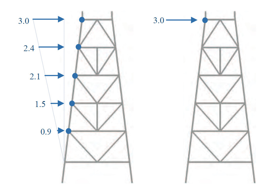Figure  26  Two types of distribution of lateral displacement applied in FE models

Download: Full-Size Img

Almost all the elements were defined by yield stress of 355 MPa and ultimate strength of 535 MPa at a plastic strain of 0.144. The values of true stresses and logarithmic strains are calculated from the nominal experimental values.

Figures 27 and 28 present the results of the pushover analysis performed on the two separate steps explained before. In Figure 27 the distribution of lateral displacement which defined in FE model is triangular and has ascending order in height with a maximum displacement of 3 m in the main deck. While Figure 28 illustrates the results of pushover analyzes with a point-centered lateral displacement of 3 m at the level of main deck. Both of distributions are in accordance with pictures shown in Figure 26.

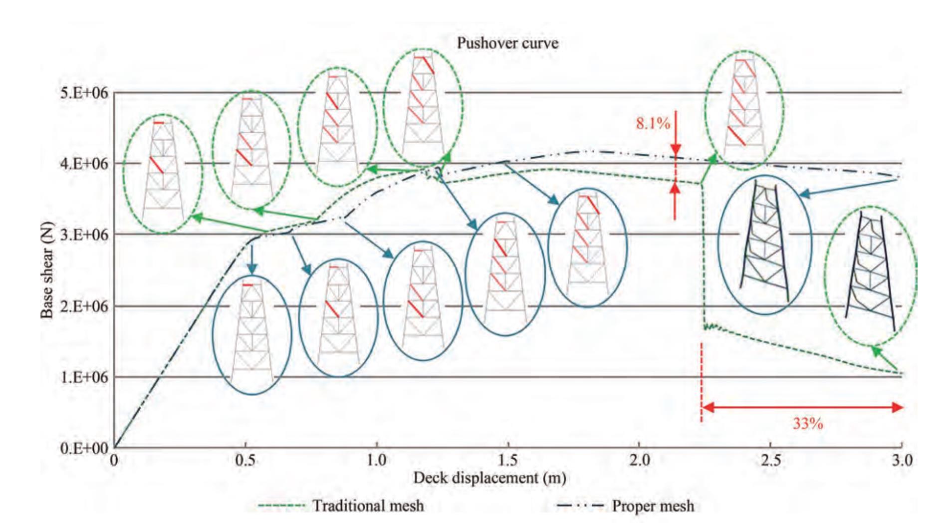Figure  27  Results of Pushover analysis of models with improper and proper mesh for push distribution type 1

Download: Full-Size Img

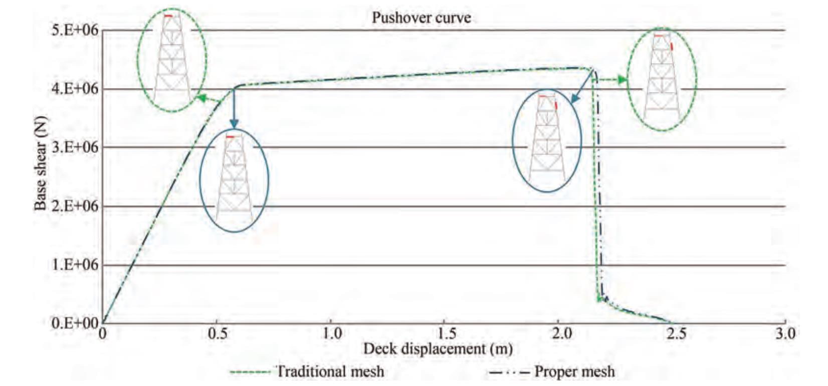Figure  28  Results of Pushover analysis of models with improper and proper mesh for push distribution type 2

Download: Full-Size Img

The order of buckling occurrence in braces is displayed in the Figure 27. The buckling of the compressive brace positioned at the lowest level of the jacket causes immediate drop and severe loses of global capacity throughout the structure. The buckling of this brace did not observe when proper mesh was assigned to all braces. Therefore, a sharp drop in pushover capacity curve has not occurred in models with proper mesh. According to the Figure 27 applying improper mesh size for compressive members can under-predict the ductility by 33% and under-estimate the lateral loading capacity up to 8%.

As seen in Figure 28 the point-centered lateral push of jacket, did not actuate the compressive capacity of braces and no buckling can be seen in the braces of jacket. Finally, only damage occurrence in the pile at top level causes immediate resistance loss and global collapse of the structure. So, at this loading distribution, results of models with proper and improper mesh size are almost similar and cannot be distinguished from each other.

Furthermore, below diagrams have been addressed to distinguish how other parameters influence the pushover results in this case study of a jacket structure.

As shown in above diagrams of Figures 29 and 30, the critical buckling load has been affected by imperfection and the element types and mesh size have a great influence on the occurrence of local buckling and the amount of strength reduction after buckling.

Figure  29  Comparison of Pushover results of models provided with various effective parameters including imperfection and element type for push distribution type 1

Download: Full-Size Img

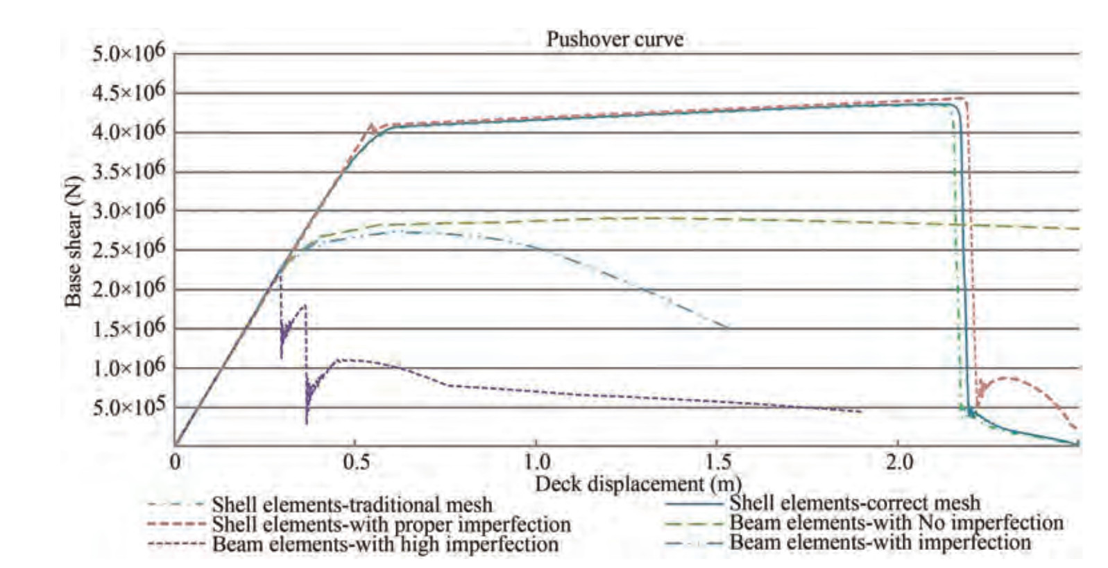Figure  30  Comparison of Pushover results of models provided with various effective parameters including imperfection and element type for push distribution type 2

Download: Full-Size Img

Figure  31  Local stresses contours in braces and beams at the end of the pushover analysis

Download: Full-Size Img

Also, the local stresses contours on deformed plots of compressive beams and braces of jacket have been illustrated bellow.

8   Conclusion

In summary, the following points can be mentioned according to the results derived from three experimental verifications, results of models, and one case study of a jacket frame. Some of these outcomes were obtained from FE models, but their accuracy was confirmed by comparing with experimental results.

1) If the buckling occurs the most accurate buckling load can be estimated by the least imperfection.

2) As the D/t ratio increases in short members, the disagreement rate between model results and the true critical buckling load increases significantly but in greater lengths (L/D ratio higher than 30), the rate is not significant.

3) The interaction between local and global buckling can lead to a drop in load carrying capacity and according to experimental results, this interaction can occur in D/t ratios of 60 and above.

4) Concerning the kneeling phenomenon (plastic local buckling occurrence) resulting drop in load carrying capacity immediately after buckling, the mesh size along the length of member is much more effective than the number of mesh elements on the cross-section.

5) Mesh element size on cross-section does not affect the elastic stiffness in compressive behavior of a tubular member.

6) Increasing the mesh size ratio can lead to more disagreement between model results and the ISO equation.

7) Adopting more than 32 mesh elements will only increase the computational cost and the run time and no significant changes in the buckling and post-buckling results will occur.

8) According to comparison of FE models by experimental result, it can be concluded that the mesh size ratio (diameter-to-thickness ratio) alone has no effect on buckling of member. But choosing values greater than 1/3 for it may cause no local buckling occurrence in the member and consequently the post-buckling strength may increases incorrectly.

9) Mesh ratio is introduced as the most effective parameter on the accuracy of elastic stiffness and post-buckling strength. Similarly, the imperfection parameter is significantly the most important factor regarding to calculation of the critical buckling load.