1   Introduction

Tubular members, because of their high capacity and convenient equipment installation, are extensively used in the support system of offshore structures such as jackets and jack-ups (Lu et al., 2020). These tubular structural members are connected by the welding process which leads to tubular joints. As an intrinsic feature of a tubular joint, the local joint flexibility (LJF) is one of the factors affecting the dynamic response and global static of an offshore structures. The LJF decreases the buckling loads, increases the deflections, changes the natural frequencies, and redistributes the nominal stresses of the structure (Ahmadi and Mayeli, 2018; Underwater Engineering Group, 1985; Bouwkamp et al., 1980). Consequently, the conventional methods for the analysis and design of the tubular joints may not be reliable enough. Because, they assume that the joints are rigid. This local deformation would decrease the capacity of the joint by redistributing the member-end moments and loads compared with the usual rigid joint. This results in reducing the cost (Gao et al., 2013; Nassiraei, 2017). Hence, it is important to investigate the LJF of tubular joints with a reliable method.

Khan et al. (2016 and 2018), Asgarian et al. (2014), Fessler et al. (1986), Buitrago et al. (1993), Nassiraei and Yara (2022) indicated that ratio of the chord dimeter to brace diameter (β), the ratio of chord radius to chord thickness (γ), the ratio of brace thickness to chord thickness (τ), and the brace angle (θ) have the most influential parameters in joint flexibility of K-joints. Also, Nassiraei and Rezadoost (2021a) showed that the reinforcing plate thickness and length have effect on the joint flexibility of joints reinforced with the reinforcing plates.

In this paper, firstly, a numerical model was created and validated with the results of 16 experimental tests. In the numerical models, the weld connecting the brace to the chord was generated. In the next step, a set of 150 K-joints (Figure 1) was numerically simulated to investigate the effect of the reinforcing plate size (η and λ), the joint geometry (β, ξ, γ, and τ), and the brace angle (θ) on the f_LJF of the reinforced joints (f_{LJF, s}) and the ratio of the f_{LJF, s} to the f_LJF of the corresponding un-reinforced joint (f_{LJF, u}). The parameters (η, λ, γ, θ, β, τ, and ξ) are applied to relate the f_LJF of the reinforced K-joint. The parameters are shown in Figure 1. After investigating the effect of each parameter on the f_LJF, a detailed f_LJF database was prepared and fi nally, a parametric equation was derived. It can be safely utilized for constructing and reinforcing the joints in offshore structures.

Figure  1  K-joint reinforced with the outer plate

Download: Full-Size Img

2   Literature review

No study is carried out on the LJF in K-joints with any methods under axial load. However, some works are conducted on the LJF in un-reinforced K-joints. Fessler et al. (1986a) assessed the f_LJF in un-reinforced multi-brace tubular joints. Asgarian et al. (2014) and Buitrago et al. (1993) studied the LJF of K-joints. In these works, just one brace was subjected to force. In addition, Khan et al. (2016) compared past studies on the f_LJF in un-reinforced K-joints. Chen et al. (1990) established some equations to determine the f_LJF in CHS K-joints.

Nassiraei and Yara (2022) investigated the effect of the external plate on the f_LJF in K-joints under bending loads. Nassiraei and Rezadoost (2021b) investigated the effect of the external plate and fiber reinforced polymer on the f_LJF in joints. Also, they established some equations for calculating the f_LJF. Furthermore, some other works are carried out on the static capacity of tubular T- and X-joints reinforced with the external plates. Li et al. (2018), Ding et al. (2018), and Zhu et al. (2017) showed that the reinforcing plate can increase the ultimate strength of X- and T-joints. Also, other methods can be used for reinforced tubular joints, such as collar plates (Nassiraei et al. 2018; Nassiraei et al. 2019; Nassiraei 2019a), doubler plates (Nassiraei et al. 2016; Nassiraei et al. 2017), fiber reinforced polymers (Nassiraei and Rezadoost 2021c; Nassiraei and Rezadoost 2021d; Nassiraei and Rezadoost 2021e; Nassiraei and Rezadoost 2021f), and external ring (Nassiraei and Rezadoost 2022a; Nassiraei and Rezadoost 2022b).

Fessler et al. (1986b) conducted several experimental Tand Y-models under axial, OPB, and IPB loads. They established some equations for determining the f_LJF. Also, the LJF in T/Y-joints was studied by Efthymiou (1985). Martins and Silva (2015) investigated the effect of LJF on the offshore structure behavior. Also, the works of Mishra et al. (2021), Kumar et al. (2015), Chaubey et al. (2018a), and Chaubey et al. (2018b) can be mentioned.

It can be concluded from the preceding paragraphs that the effect of none of the reinforcing techniques on the f_LJF in K-joints under axial load has been investigated. Consequently, there is an essential requirement for investigating so that concrete guidelines on LJF evaluation in retrofitted K-joints with the external plates can be formulated. Figure 1 presents a K-joint reinforced with the external plates. This retrofitting technique can be applied to structures during design and operation.

3   Definition of the f_LJF

For the joins under axial load, the LJF can be defined as:

where P is the brace load, Δ is the average local deformation normal to the chord axis. It can be determined by Eq. (2). Also, the θ is the brace angle (Figure 1).

The positions of Δ₁ - Δ₄ and Δ'₁ - Δ'₄ are showed in Figure 2. For relating the LJF to the joint's geometry, a coefficient named the f_LJF is defined. For the tubular K-joints in axial load, the f_LJF can be obtained using Eq. (3).

Figure  2  Points of measured deformation on the joint

Download: Full-Size Img

where, E is Young's modulus.

4   FE modeling and validation

ANSYS Ver. 20 was used for the numerical simulation. The recommendations of AWS (2005) were utilized to design the welds, as previous works (Nassiraei and Rezadoost 2020; Nassiraei and Rezadoost 2021g; Nassiraei and Rezadoost 2021h). The generated weld can be seen in Figures 1 and 3 (red color). To mesh of the chord, welds, braces, and plates, the SOLID185 element was applied. Figure 3 depicts a meshed K-joint with the external plates. In Figures 3 and 4, the stiffener plates are shown in blue color. The balanced loads were applied to the brace ends (Figure 1a). Also, the displacements of the chord ends were fixed. Moreover, the linear static analysis was used to obtain the f_LJF (Nassiraei 2020; Nassiraei 2022). Also, Lostado Lorza et al. (2015), Lostado Lorza et al. (2018), 2017, and Íñiguez Macedo et al. (2019) were used to solve some of the key questions and points for meshing and boundary conditions.

Figure  3  Generated mesh in the reinforced K-joint: (a) Reinforced joint, (b) and (c) Joint intersection and (d) weld profile

Download: Full-Size Img

Figure  4  Mesh details and boundary conditions

Download: Full-Size Img

Until now, no experimental data of f_LJF for K-joints with any reinforcing method is available. Therefore, bellow experimental data are utilized to confirm the present FE model:

• The f_LJF of 11 T/Y-joints under axial load

• The load-displacement curve of two X-joints reinforced with the external plates under tension

• The force-displacement curve of two X-joints with the external plates under compression

• The load-displacement curve of one T-joints with the external plates under compression The joint properties have been tabulated in Table 1. Also, the material properties of the members are tabulated in Table 2.

The numerical, experimental, and empirical f_LJF values of the 11 un-reinforced T, and Y-joints subjected to axial load are listed in Table 3. Mean Absolute Error (MAE) and Root Mean Square Error (RMSE) are 8.7 and 13.04, respectively. The comparison (Table 3) shows that the f_LJF values of the FE models are close to the corresponding f_LJF values of the experimental and empirical models. Consequently, the current developed numerical model precisely estimates the f_LJF of tubular joints in axial load. Figure 5 indicates the load-displacements curves of tubular X- and Tshaped joints reinforced with the external plates under axial load. The result shows that the initial joint stiffness of the FE models and experimental tests is very close, for all the reinforced tubular joints. Moreover, the present study of f_LJF in the joint is within the elastic range, the same as previous works (Nassiraei 2019). Consequently, the present numerical model of the reinforced tubular joints is accurate enough to generate safe f_LJF results.

Figure  5  The comparison the present numerical results with the experimental data

Download: Full-Size Img

5   Effect of geometrical parameters on the f_LJF and ψ

5.1   Details

One hundred fifty numerical models were generated, in ANSYS version 20, to investigate the effect of the brace angle (θ), joint geometry (τ, ζ, β, and γ) and the reinforcing plate (η and λ) on the f_LJF of the reinforced K-joints under axial load. The definition of the parameters is presented in Figure 1. The numerical models include three diverse η ratios, three different λ ratios, seven different τ proportions, five different θ ratios, five different ζ ratios, seven different γ ratios, and seven different β ratios. The elastic module of Young for the members and weld equals 207 GPa. To investigate the f_LJF of the reinforced K-joints with the corresponding un-reinforced joints, a new parameter χ is presented. The χ is defined to f_{LJF, s}/f_{LJF, u}. The f_{LJF, s} is the f_LJF of the K-joint reinforced with the reinforcing plate. The f_{LJF, u} is the f_LJF of the un-reinforced K-joint.

5.2   The effect of θ, η, and λ

Figure 6 shows that the increase of the θ leads to the increase of the f_LJF. Because, the increase of the θ leads to the decrease of the initial joint stiffens. Also, the external plates have considerable effect on decreasing the f_LJF. Because in the reinforced joints, the reinforcing plates enhance the joints stiffness. The increase of the joint's stiffness leads to the decrease of the reshaping. Furthermore, the results indicate that the effect of the reinforcing plate thickness on the decrease of the f_LJF is more significant than the effect of the reinforcing plate length on the decrease of the f_LJF. Because, the main displacement happens in the joint intersection. Hence, using the reinforcing plate with more length cannot be very useful. Also, in the K-joint with bigger θ, the reducing effect of the stiffener plate on the f_LJF becomes more considerable. For example, in the reinforced joints with η = 3, λ = 3, γ = 18, β = 0.7, ξ = 0.4, and τ = 0.8, when the θ is 30°, 45°, and 60° the χ (f_LJF ratio of the reinforced to the corresponding un-reinforced joints) is equal to 0.59, 0.44, and 0.30.

Figure  6  The effect of the θ, λ, and η on the f_LJF and the χ (f_LJF ratio of the reinforced to the corresponding un-reinforced joint) for the joints with τ = 0.8, ξ = 0.4, γ = 18, and β = 0.7

Download: Full-Size Img

5.3   The effect of β, η, and λ

This section studies the effect of the β, η, and λ on the f_LJF and the χ in the joints with γ = 32, ξ = 0.3, τ = 0.5, and θ = 40°. Figure 7 illustrates that the increase of the β leads to the decrease of the f_LJF. Since, the brace diameter and the reinforcing plate length in the reinforced joints with higher β are bigger than the brace diameter and the reinforcing plate length in the corresponding reinforced joints with smaller β, respectively. The growth in these two parameters leads to the increase in the initial joint stiffness. In addition, the f_LJF of the reinforced K-joints is notably smaller than the f_LJF of the corresponding un-reinforced Kjoints. Also, by decreasing the β value, the effect of the λ and η value on the f_LJF and χ become more significant. For example, in the joints with η = 1, λ = 2, γ = 32, ξ = 0.3, τ = 0.5, and θ = 40° (Figures 7d-7f) the χ for the joints with β = 0.2, 0.5, and 0.8 is equal to 0.72, 0.87, and 0.91 respectively. As a result, the enhancing effect of the reinforcing plate is more significant for the joints with smaller β.

Figure  7  The effect of the β, λ, and η on the f_LJF and the χ (f_LJF proportion of the reinforced to the corresponding un-reinforced joint) for the joint with ξ = 0.3, τ = 0.5, γ = 32, and θ = 40°

Download: Full-Size Img

5.4   The effect of γ, η, and λ

This section investigates the effect of the γ, λ, and η on the f_LJF and the χ. Figure 8 presents the results for the joints with ξ = 0.5, β = 0.3, τ = 0.6, and θ = 50° and different values of the γ, η, and λ. As it can be seen, the f_LJF of the un-reinforced joints is remarkably bigger than the f_LJF of the corresponding plate-reinforced joints. Also, by increasing the reinforcing plate size, the difference between the f_LJF of the un-reinforced and reinforced joints becomes bigger. Since, the bigger stiffener plates absorb more energy. Consequently, using the bigger plates leads to less reshaping and f_LJF. However, the effect of the reinforcing plate thickness on decreasing the f_LJF is more remarkable than the effect of the reinforcing plate length on decreasing the f_LJF.

Figure  8  The effect of the γ, λ, and η on the f_LJF and the χ (f_LJF proportion of the reinforced to the corresponding un-reinforced joint) for the joint with ξ = 0.5, β = 0.3, τ = 0.6, and θ = 50°

Download: Full-Size Img

The results indicate that the increase of the γ leads to the considerable decrease of the f_LJF. Because, the increase of the γ leads to the decrease of the thicknesses in both the chord and external plates. This results in the decrease of the joint stiffness. But, the effect of the γ on the χ can be ignored. For example, in the joints with η = 2, λ = 3, ξ = 0.5, β = 0.3, τ = 0.6, and θ = 50°, the χ is equal to 0.49 and 0.51 for the joints with γ equal to 15 and 20, respectively.

5.5   The effect of τ, η, and λ

This section investigates the effect of τ, λ, and η on the f_LJF and χ in the joint with ξ = 0.2, β = 0.4, θ = 45°, and γ = 25. Figure 9 indicates that LJF of the reinforced joints is notably smaller than the corresponding un-reinforced joints. For instance, the f_LJF of the reinforced joints with η = 2, λ = 2, τ = 0.7, β = 0.4, γ = 25, θ = 45°, and ξ = 0.2, (Figure 9e) is 59% of the f_LJF of the corresponding un-reinforced joints. Furthermore, the increase of the τ leads to the decrease of the f_LJF. Since, the increase of the τ leads to the increase of the brace thickness. The growth of this thickness results in the enhancement of joint stiffness. As it can be concluded, the change of the τ from 0.4 to 0.7 can result in more decrease in f_LJF rather than the change of the τ from 0.7 to 1.0.

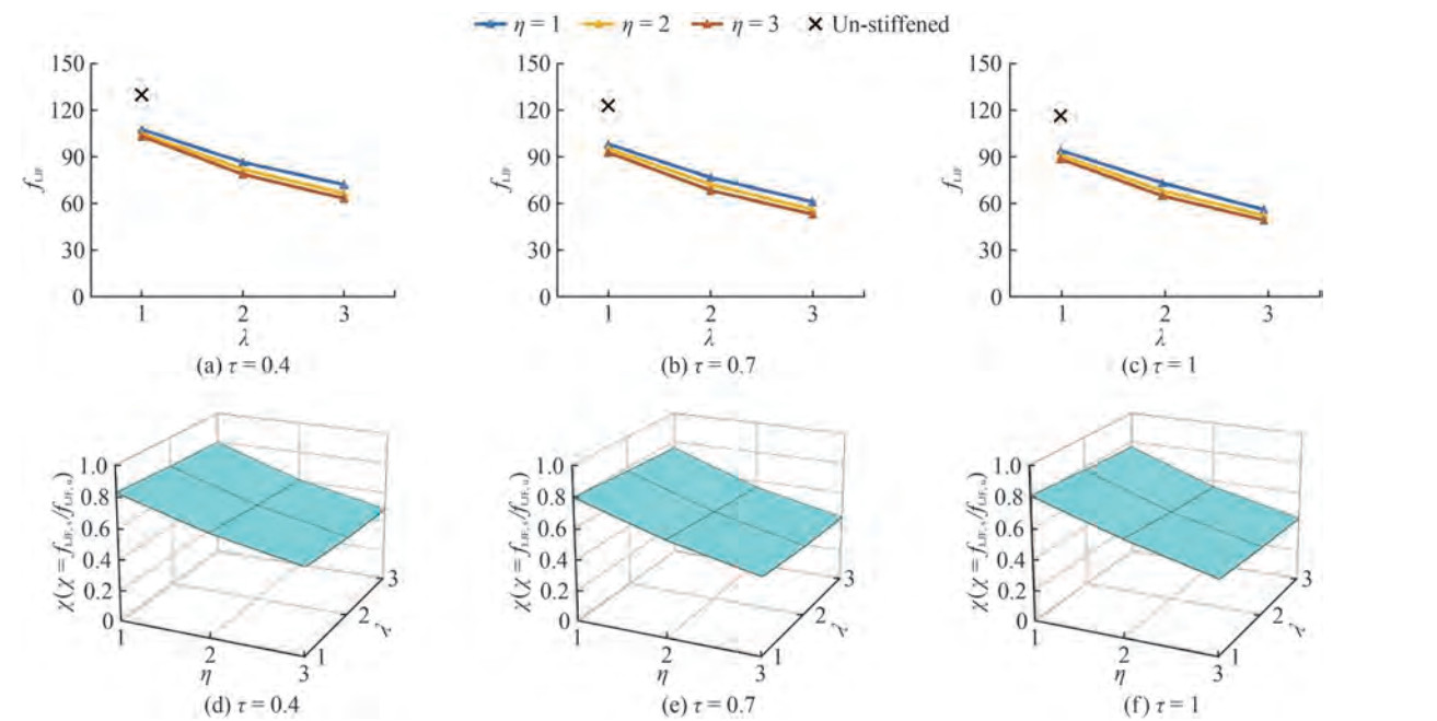Figure  9  The effect of the τ, λ, and η on the f_LJF and the χ (f_LJF proportion of the reinforced to the corresponding un-reinforced joint) for the joint with ξ = 0.2, γ = 25, β = 0.4, and θ = 45°

Download: Full-Size Img

5.6   The effect of ξ, λ, and η

Figure 10 shows the ψ values for the joints with different values of the ξ, η, and λ. It can be observed that the increase of the ξ leads to a slight decrease of the ψ. For example, in the joints with η = 1, λ = 3, γ = 12, β = 0.9, τ = 0.9, and θ = 60, when the ξ is equal to 0.2, 0.4, and 0.6, the ψ is equal to 0.69, 0.67, and 0.65, respectively. Despite the ξ, the increase of the reinforcing plate size (η and λ) leads to the significant decrease of the ψ.

Figure  10  The effect of the ξ, λ, and η on the f_LJF and the χ (f_LJF proportion of the reinforced to the corresponding un-reinforced joint) for the joint with γ = 12, β = 0.9, τ = 0.9, and θ = 60°

Download: Full-Size Img

6   Design formula

No formula is available to determine the f_LJF in reinforced K-joints under axial load. Therefore, by using the obtained data of the current 150 FE models and SPSS (software package), parametric Eq. (5) is proposed for this aim.

In order to develop this parametric equation, multiple nonlinear regression analyses were performed by the statistical software package, SPSS. Values of dependent variable (i.e. f_LJF ratio) and independent variables (λ, η, θ, γ, β, and τ) constitute the input data imported in the form of a matrix. Every row of this matrix involves the information about the f_LJF ratio values in a reinforced K-joint having specific geometrical properties. The input matrix for derivation of the equation had 150 rows equation (the number of FE models) and 7 columns (equation the number of dependent and independent variables). Hence, the whole FE strength ratio database was arranged as 1 400 input matrices. When the dependent and independent variables are defined, a model expression must be built with defined parameters. Parameters of the model expression are unknown coefficients and exponents. The researcher must specify a starting value for each parameter, preferably as close as possible to the expected final solution. Poor starting values can result in failure to converge or in convergence on a solution that is local (rather than global) or is physically impossible. Various model expressions must be built to derive a parametric equation having a high coefficient of determination.

where χ is the f_LJF ratio of the retrofitted K-joints to the corresponding un-retrofitted joint under axial load. The R² is the determination factor. Its value is close to 1. The application range for the use of Eq. (4) is as follow:

If consider P and M as the predicted values and the measured value, respectively, the UK Department of Energy suggests the below standard.

• If [P/M < 0.8] ≤ 5%; and [P/M < 1.0] ≤ 25%, the formula is accepted. If also, [P/M > 1.5] ≥ 50%, the equation is taken as commonly circumspect.

• If 5% < [P/M < 0.8] ≤ 7.5%, and/or 25% < [P/M < 1.0] ≤ 30%, the formula is taken as borderline. consequently, more evaluation should be conducted.

• Otherwise, the established equation cannot be approved. Because, it is too optimistic.

It should be noted that according the recommendation of Bomel Consulting Engineers (1994), P/R < 1.0 can be eliminated in the assessment. Evaluating Eq. (4) according to the UK DoE (1983) standard is listed in Table 4. It can be seen that the equation needs revision. To revise Eq. (4), the f_LJF, s values calculated from the equation was multiplied by a factor in such a way that resulted f_LJF, s values satisfying the UK DoE (1983)acceptance standard. The design factor can be determined as follows:

where the values of f_{LJF, s (Eq. (4)} are calcula ted from the derived equation and the values of f_{LJF, s (Design)} are expected to satisfy the UK DoE (1983) standard. The following formula is suggested for the design aims.

The results of the evaluation for the revised equation based on the UK DoE (1983) standard are tabulated in Table 4.

Mean Absolute Error (MAE) and Root Mean Square Error (RMSE) are 0.03 and 0.04, respectively. In Figure 11, the f_LJF ratios extracted by the proposed equation are compared with the corresponding values obtained from FE analyses. The value of R² (R² = 0.91), evaluating the equations based on the UK DoE standard, and Figure 11 indicate that the proposed formula is accurate to produce reliable data.

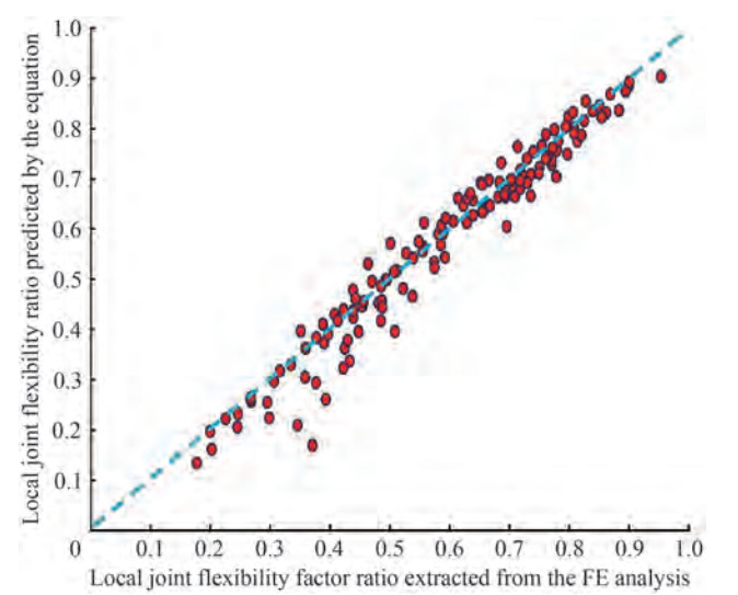Figure  11  Comparison of the χ (f_LJF ratio) predicted by the proposed formula with the associated values extracted from the FE models for the stiffened K-joint

Download: Full-Size Img

7   Conclusions

A total of 150 numerical models, after validation with several experimental tests, was generated to investigate the effect of the joint geometry, the brace angle, and the stiffener plate size on the f_LJF of the tubular K-joints under axial load. The main conclusions are as follows:

• Verification of the present numerical models with experimental results indicates that the FE model can well predict the f_LJF of un-reinforced and plate reinforced K-joints in axial loads. In addition, the reinforcing plate thickness and the reinforcing plate length have significant effect in the decrease of the f_LJF.

• The results indicated that using the external plates can decrease 81% of the f_LJF.

• The increase of the θ results in the increase of the f_LJF. Moreover, in the joints with bigger θ, the reducing effect of the stiffener plate on the f_LJF becomes more significant.

• The increase of the β leads to the decrease of the f_LJF. Because, the brace diameter and the reinforcing plate length in the reinforced joints with higher β are bigger than the brace diameter and the reinforcing plate length in the corresponding joints with smaller β, respectively. The growth in these two parameters leads to the increase in the joint stiffness. Also, by decreasing the β value, the effect of the λ and η value on the f_LJF and f_LJFratio (χ) becomes more considerable. Consequently, the reinforcing effect of the reinforcing plate is more remarkable for the joints with smaller β.

• The increase of the γ leads to the considerable decrease in the f_LJF. Because, the increase of the γ leads to the decrease of the thicknesses in both the chord and external plates. However, the effect of the γ on the χ can be ignored. The increase of the ξ leads to a slight decrease of the χ. The increase of the τ leads to the decrease of the f_LJF in the reinforced joints.

• A design formula is proposed for determining the f_LJF in K-joints reinforced with the external plates under axial load. High determination factor (R² = 0.91), accepting the UK DoE criteria, and good match compared to corresponding values in a figure indicted that the proposed formula can be reliably utilized for designing and reinforcing tubular K-joints.