1   Introduction

Jacket-type offshore platforms, commonly used in the oil industry, are usually fabricated with tubular joints. In operation, these structures are generally subjected to cyclic stresses which usually result in fatigue fractures (Visser 1974). Moreover, their geometrical structures are usually made up of different shapes of tubular structures joined by welding to form tubular joints (Arsem, 1987). The tubular joints play a major role in securing the structural elements. Thus, these structures are either floating or mobile and are designed to withstand residual stresses and external stresses such as tides, storms, swells, currents and winds (API, 1993). In addition, they must be able to resist the corrosion associated with this environment, as well as the seismic risk (Bellagh, 2001). The complex intersections of these joints represent structural discontinuities leading to high stress concentrations near the welds. These high stress concentrations typically cause fatigue failure of welded tubular joints on offshore platforms that are subjected to cyclic loading in corrosive marine environments (Mohamad, 2007). Therefore, an accurate assessment of the magnitude of stress concentrations is necessary to properly address the problem of fatigue damage and to manufacture more reliable tubular joints (N'Diaye et al., 2007).

A great deal of research has been carried out on various aspects to evaluate the fatigue life of welded tubular joints in particular the stress concentration factor (SCF) is one of the most important factors to evaluate the safety of the tubular joints (Efthymiou, 1988; Lloyd's, 1992). The aim of this work is the determination of parametric equations for calculating the SCF so that the practising engineer can use them to obtain the strongest tubular joints (Chang and Dover, 1996). In addition, the authors analyzed several studies on the mechanical behavior under different loading and boundary conditions on various types of tubular joints. Kuang et al. (1975), Wordsworth (1981), Efthymiou and Durkin (1985), Hellier et al. (1990) and Smedley and Fisher (1991) have made important contributions in their respective works to the determination of the SCF for different loading configurations. In addition, they proposed parametric equations for various geometrical configurations, in particular those for tubular T, Y, K, KT and X-joints. Lee and Wilmshurst (1995) and Lee (1999) present the modelling techniques used in the finite element analysis of tubular K-joints to obtain information on strength, stress fields and stress intensity factors. The numerical results were rigorusly calibrated against existing experimental data. Cao et al. (1997) in their work explain the mesh generation for different types of welded circular tubular joints with or without cracks for finite element analysis. Furthermore, their methods can be applied to different types of joints, uniplanar or multiplanar, uncracked or cracked, and high quality meshes can be obtained using this method. Morgan and Lee(1998a, 1998b) presented a set of parametric equations for determining the SCFs of tubular K-joints under balanced axial and out-of-plane bending loading respectively. The equations were developed using a database of thin shell finite element results and allow the estimation of SCFs at key locations on the brace-chord intersection. Gandhi et al. (2000) in their work develop a model for estimating the lifetime of crack initiation and growth by performing constant amplitude corrosion fatigue tests on internally ring-stiffened steel tubular T and Y-joints under freely corroding conditions. Hoon et al. (2001) present a study of a large-scale round-to-round tubular T-joint reinforced with a doubler-plate under the combined action of three types of base loads. Their work shows that the maximum hot spot stress is located on the doubler plate, equivalent to the chord of an unreinforced joint, for all base loads and combined loads. Gao (2006) and Gao et al. (2007) presented a set of parametric equations for determining the SCFs in fully overlapped tubular K(N)-joints under out-of-plane and in-plane bending loading by overlap, respectively. Fricke et al. (2008) in their work describe the different modelling techniques used to determine the structural hot spot stresses and the effective stresses in the notches in rectangular hollow-section T-joints. Shao et al. (2009) present the evaluation of the fatigue life of tubular K-joints under cyclic loading. In addition, they establish a set of parametric equations for calculating the stress distribution of the tubular K-joint under axial loading, in-plane bending and out-of-plane bending respectively using a curve fitting technique. Ahmadi et al.(2011a, 2011b, 2012a), Ahmadi et al. (2012b) and Ahmadi and Lotfollahi-Yaghin(2012c, 2013) present the effects of geometrical parameters on stress concentration factors in uniplanar, multiplanar and internally ring-stiffened KT-joints under axial loads. In addition, the effects of stress concentration factors on the fatigue reliability along the weld toe of uni-planar and multi-planar tubular DKT-joints respectively are investigated. They determine the probability distribution describing the stress concentration factors in tubular joints, especially multi-planar DKT-joints, in order to study the effect of these parameters on the reliability analysis results. Yang et al. (2015) present measurements of the elastic gradient strain distributions along the intersection of tubular N-joints. In addition, a set of parametric equations taking into account the eccentricity ratio was proposed to calculate the SCFs of tubular N-joints with large negative eccentricity based on the computational results of numerical models. Liu et al. (2015) in their work on tubular T-joints, present the improved Zero Point Structural Stress (ZPSS) approach for calculating the structural stress for fatigue life assessment of tubular joints. Parametric equations with a high degree of fit for the calculation of the stress concentration factor are derived on the basis of the ZPSS approach for the stress analysis of tubular T-joints in engineering. Ahmadi and Lotfollahi-yaghin (2015), Ahmadi and Zavvar (2015) and Ahmadi and Nejad (2016) have shown in their work that stress concentration factors play a crucial role in assessing the fatigue performance of tubular K and KT-joints under in-plane and out-of-plane bending loads. Moreover, Ahmadi et al.(2015, 2016) and Ahmadi (2016) present the probability distribution of stress concentration factors, especially for internal ring reinforced tubular KT-joints under axial, in-plane bending and out-of-plane bending sub-loads respectively. However, probability distribution models for the stress concentration factors in internal ring reinforced tubular KT-joints have been proposed. Cao et al. (2018) present a parametric study of stress concentration factors (SCF) on tubular X-joints used in offshore platform structures. It was found that the influence of residual welding stress is negligible on the analysis of SCF values in tubular joints. Iberahin (2018) and Iberahin and Talal (2019) in their work on the analysis of SCFs under axial loading and out-of-plane bending on the tubular K-joint, show that the effect of dimensionless parameters on SCFSs depends on the type of loading. Sambo et al. (2022) in their work present the effects of dimensionless parameters on the stress concentration factor in tubular TY-joint under axial loads. Furthermore, they establish parametric equations to calculate the stress concentration factor that can withstand fatigue phenomena.

However, in the majority of the literature, stress concentration factors are one of the most influential factors in the fatigue strength of tubular joints (Vincent, 2011). This is justified by a large number of works on stress concentration factors on different shapes of tubular joints. Although tubular TY-joints are commonly used in offshore jacket structures, stress concentration factors on TY-joints under in-plane bending (IPB) and out-of-plane bending (OPB) loads have not been addressed in this case.

In this work, study of the stress distributions in the vicinity of the intersection lines of the tubular elements and the location of hot spots stress at critical locations in tubular TY-joints are studied. To the best of our knowledge, this configuration for SCF determination in tubular TY-joints cannot been found in the literature. This analysis is performed by the finite element method on 81 generated models of the tubular TY-joint subjected to in-plane bending (IPB) and out-of-plane bending (OPB) loading conditions using Comsol Multiphysics software. The study consists to analyze the influence of geometrical parameters on the SCF in the case of IPB and OPB loads, around the weld toe for TY-joints. The results of the finite element analysis allow us to establish new parametric equations for the calculation of the SCF at fatigue critical locations, using the non-linear regression method.

2   Finite element modeling

The use of a numerical method via software (Comsol Multiphysics) proved to be one of the best solutions given the difficulty of experimental measurements. For this purpose, the finite element method is the best suited to the constraints imposed by the problem (Shao, 2004). However, the finite element method has emerged as one of the most widely used general methods for structural analysis.

2.1   Geometric parameters of the tubular gap TY-joint

In this work, we analyze the behavior of tubular gap TYjoints (illustrated in Figure 1) subjected to IPB and OPB loads. This tubular joint is found in various structures, in particular in offshore jacket structures. It has a circular cross-section and consists of two braces connected to the chord by welding. One of the braces is vertical and the other is inclined at an angle of θ < 90° with the chord. However, gap of the vertical brace and the inclined brace is defined as the distance between the welding points of the two braces of the tubular gap TY-joint. In order to improve the constructability of the tubular gap TY-joint, it is necessary to determine the appropriate length of gap brace to reduce the stress concentration. Thus, seven models with different values of the length of gap brace were constructed in order to evaluate its effect on the hot spot stress as shown in Table 1. According to Table 1, the effect of the length of gap brace on the hot spot stress values is almost negligible. As demonstrated in the work of Ahmadi et al (2011a). Therefore, a typical value of the gap parameter ζ = 0.15 is assigned to all our models.

Figure  1  Geometric representation of a tubular gap TY-joint

Download: Full-Size Img

To avoid an impact on the stresses observed at the chord/ brace intersection in order to obtain good information on the stress concentration value, the length of the chord must be really long. Thus, Efthymiou (1988) in his work explained that this impact can be affected by the boundary conditions applied at the chord levels. However, in order to choose a suitable value for the chord length parameter α, six models were constructed to study the effect of this parameter on the SCF. Therefore, the results of this partial study have been presented in Table 2. From this analysis on the six models with different values of α given in Table 2, it appears that the value of this parameter has no effect on the values of the SCF. A realistic value of α = 12 is assigned in all models in the current study.

The brace length must be well defined so that the determination of the stress concentrations is not affected by the boundary conditions. However, Chang and Dover (1999) showed that the brace length parameter αB does not have much influence on the hot spot stress when the value of α_B exceeds the threshold value. Thus, in the present study, a realistic value of α_B = 8 is used for all models in the current study in order to have an appropriate brace length. Steel with a Young's modulus of 207 GPa and a Poisson's ratio of 0.3 was used as the material for our model.

The geometric parameters used in this work are summarized in Table 3. These geometrical parameters cover the actual practical values commonly found for the realization of tubular joints in offshore platform structures. Moreover, these geometrical values are similar to the one proposed by Sambo et al. (2022). Depending on the values of γ, τ and β of each joint, the diameter and wall thickness parameters of the brace are changed from one design model to another.

2.2   Calculation of the SCFs

The tubular joint has a specific geometry, which results in high stress concentrations near the welds toe. Under repeated loading, these concentrations lead to the creation of cracks, which can become large enough to cause the joint to fail. The location of the maximum stress concentration is called a hot spot. The location of the hot spots, where the SCF values are highest and which are preferred sites for fatigue crack initiation, is important in assessing the service life. Therefore, it is important to accurately determine the distributions of SCF values near the intersection lines of the tubular joints.

Several methods are used to obtain the hot spot stress of tubular joints, in particular that of the IIW (1999). Due to the nature of the stress field in a hot spot region, recent research on how to establish the hot spot stress (see Figure 2) is established (DNVGL-RP-C203, 2016). The hot spot stress is derived by extrapolating the structural stress to the end of the weld, as shown in Figure 2. It is noted that the stress used as a basis for such extrapolation must be outside that affected by the weld notch, but close enough to capture the stress due to the local geometry.

Figure  2  Representation of the method for obtaining the hot spot

Download: Full-Size Img

According to the illustration in Figure 2, the stresses at points A and B, which lie within a specified extrapolation region, are first determined by using the finite element analysis in Ref. DNVGL-RP-C203 (2016). The hot spot stress is then calculated by extrapolating the stresses at points A and B linearly to the end of the weld. The distribution of the hot spot stress on the weld toe is absolutely identical to the SCF as the beam theory is applied or in a direct way to calculate the nominal stress on the brace depending on the type of load. Therefore, for all FEA analyses in this work, the hot spot stress is given by the value of the Von Mises stress in the results. However, the Von Mises stress is a better parameter for the analysis (Lalitesh et al. 2018).

Therefore, the SCF of the tubular joint is defined as the ratio of hot spot stress to nominal stress and is expressed as:

where σ_hss is the hot spot stress and σ_n is the nominal stress. For in-plane and out-of-plane bending loads applied to a joint, the nominal stress σ_n is defined as follows (Shao 2004):

where j = i, o; M_i and M_o are the in-plane-bending and outof-plane bending moment respectively. Likewise, d and t are brace diameter and thickness respectively.

Figure 3 shows the distribution of stress for a tubular TY-joint subjected to the in-plane bending load.

Figure  3  Distribution of stress for a tubular TY-joint subjected to in-plane bending loading.

Download: Full-Size Img

2.3   Modeling of the weld profile

Accurate modeling of the weld profile is one of the important factors affecting the accuracy of the SCF results. This will allow us to obtain a more accurate and detailed stress distribution on the weld toe. In addition, the size of the weld toe connecting (see Figure 4b) the chord and the brace of our different tubular structures is in accordance with the AWS (2002) specifications. The weld sizes at the crown, saddle, crown toe, and crown heel positions can be determined as follows (AWS 2002):

Figure  4  Weld geometry

Download: Full-Size Img

and

where H_w and t in (mm), ψ in (deg). The expression of ψ is obtained as follows (AWS 2002):

The parameters used in Eq. (3) and Eq. (4) are defined in Figure 4.

Determination of SCFs should be carried out by modelling solid joints that include the weld, and should be based on notch stresses measured on the outer surface at the weld toe, as slight overestimations of SCFs represent a large reduction in predicted lifetimes (Lozano-Minguez et al., 2014; Hectors and Waele, 2021).

However, the use of shell elements is a common and acceptable practice for stress calculations, solid elements including the weld bead geometry are used (Schürmann and Karsten 2021).

Thus, the angle φ defining the intersection between the chord and the brace is an important parameter representing the curve along the weld toe. This angle is defined as shown in Figure 5.

Figure  5  Definition of the directional angle φ along the weld toe of tubular gap TY-joint

Download: Full-Size Img

However, the positions of the hot-spot are located according to this directional angle φ.

2.4   Mesh generation procedure and boundary conditions

In this work, the mesh used to discretize the geometry studied is of the Lagrangian type and the element used is of the triangular type. This type of element has 6 nodes (illustrated in Figure 6a). It allows the number of nodes to be increased while retaining a single nodal variable. It favours the representation of affine stress fields per element and is isoparametric because they are derived from these reference elements by a transformation that is also quadratic. However, they also have richer basis functions and therefore lead to smaller deviations from reality. In practice, experience shows that these elements generally lead to a better accuracy/cost ratio than their first order counterparts. The accuracy of the results of a finite element stress analysis depends on the elements used, the fineness of the mesh, especially in the vicinity of areas of high stress concentrations. In the area of the intersection of the chord and the strut, the mesh generated is tighter, as shown in Figure 6b. However, in finite element calculations, numerical blocking in the convergence of solutions for large shear stiffnesses is encountered in some problems. It is possible to reduce or eliminate this phenomenon by lowering the level of the interpolation functions or by introducing elements with a larger number of degrees of freedom (Ravi et al., 2022). In order to improve the performance of the element and to avoid the phenomenon of shear locking, reduced integration has been employed. The mesh convergence study was carried out in order to obtain more reliable results.

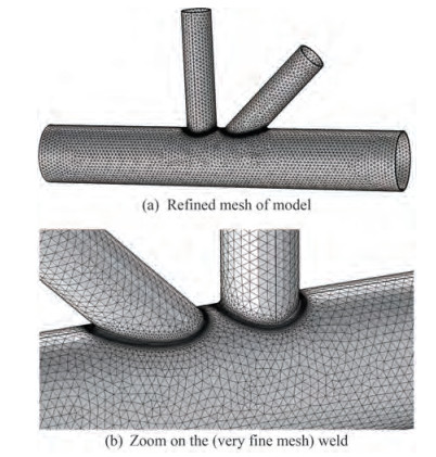Figure  6  Meshed TY-joint in COMSOL multiphysics

Download: Full-Size Img

A convergence study is performed to determine the required mesh division at which the displacement values converge as presented in the work of Ansari and Ajay(2018, 2019) and Sambo et al. (2022). Furthermore, a mesh convergence study is necessary to have more reliable results, we refined the mesh down to 3 mm on the intersection area and as CPU increases, the result converges to a constant value of 12.2 MPa (Table 4) as the maximum stress obtained under a IPB load condition 1 (Figure 7a). In addition, we performed the same convergence study in the OPB load case. Thus, the convergence of the mesh is carried out on one of the tubular joints Joint Ref. 10/1) in the UK HSE (1997) report.

Figure  7  Studied load conditions of in-plane bending and out-ofplane bending

Download: Full-Size Img

As shown in Figure 7, in this work, two different conditions of in-plane and out-of-plane bending load, respectively, are considered to determine the SCFs on the weld toe in tubular TY-joints. Figures 7a and 7b represent the balanced IPB and unbalanced IPB loads respectively.

Similarly, Figures 7c and 7d represent the balanced OPB and unbalanced OPB loads, respectively. The boundary conditions considered for all our joints designs are fixing for the both cases, to the end of the chord. The modification of the boundary conditions will change the SCF values accordingly as they are very specific values. Thus, this boundary condition allows for reduced displacements and rotations in all directions.

2.5   Validation of the finite element model

In order to validate the present finite element analysis, the accuracy of our results must be checked against the experimental test results. Thus, we compare our results with the tests carried out in the UK HSE (1997) report. The geometrical characteristics of the tubular joint (Table 5) of the steel model were chosen on the basis of the information given by the UK HSE (1997) to obtain the value of the stress concentration factors.

The results of the process verification for different types of loading are presented in Table 6. Thus, a good correlation is observed on the results of our current model with that of the equations proposed by Morgan and Lee (1998b). Moreover, these equations are used in this work for the validation of FEMs. However, the maximum difference between the results in the Table 6 is less than 10%. Thus, this difference may be due to the different modelling technique. Therefore, the finite element models generated in this work can be considered as so accurate that they provide reliable results.

3   Results

In general, offshore structures are exposed to multi-axial loadings, such as a combination of axial force, in-plane bending (IPB) and out-plane bending (OPB) moments. In this section, we can study the effects of geometric parameters β, γ, τ, and θ of the tubular TY-joints on the SCFs, due to IPB and OPB loads as illustrated respectively in Figure 7.

3.1   Effect of the parameter β on the SCFs

This subsection presents the effects of the brace-tochord diameter ratio parameter β on the SCFs and its interaction with the chord wall slenderness ratio parameter γ. In the case of the IPB loadings, our results reveal that, by increasing the values of the parameter β from 0.4 to 0.6 and setting the values of γ from 12 to 24, we observe a faint decrease of the SCFs at the toe position as depicted in Figures β 8a and 8c, respectively. We note that these values of the SCFs are observed at the weld connecting the vertical brace and the chord. In addition, an increase of the parameter by fixing the values of γ, significantly decreases the values of the SCFs, at the heel position towards the side of the inclined brace as illustrated in Figures 8b and 8d for the both loadings 1st and 2nd conditions, respectively. Therefore, our results reveal that the maximum values of the SCFs are located at the heel on the side of the chord. They represent the critical values that may be responsible of the phenomena of fatigue failure.

Figure  8  Analysis of the effect of β on the SCFs values under IPB loading

Download: Full-Size Img

In the case of the OPB loading conditions, we see that, by increasing the values of the parameter β and having constant values of the parameter γ, the values of the SCFs decreases at the saddle position as illustrated in Figures 9a and 9b, respectively. We also note that, the SCFs are observed at the weld connecting the vertical brace and the chord and have a maximum value located at the saddle position towards the side of the chord.

Figure  9  Analysis of the effect of β on the SCFs values under OPB loading

Download: Full-Size Img

In addition, the results obtained here show that, by increasing the values of the parameter β the diameter of the brace reduces the SCF in the vicinity of the intersection lines of the tubular elements. On the order hand the SCF is not dependent on either the type of IPB and OPB loadings applied or the values of the other geometrical parameters. Our results suggest that the tubular gap TY-joint is more resistant for values of 0.5 ≤ β < 1 and the parameter β is a determining factor in the stress distribution because of the way the load transfer is accomplished.

3.2   Effect of the parameter γ on the SCFs

Here, we present the influence of the chord wall slenderness ratio parameter γ, on the SCFs and its interaction with the brace-to-chord thickness ratio parameter τ, in the case of both IPB and OPB loadings. Our results reveal that, by increasing the values of γ from 12 to 24 and setting the values τ from 0.4 to 1.0, the value of the SCFs increases at the toe position as depicted in Figures 10a and 10c. Similar behavior is observed in Figures 10b and 10d at the heel position towards the side of the inclined brace. Thus, our results shown that, the maximum values of SCFs are located at the position of the heel towards the side of the chord and therefore correspond to the critical point where the fatigue strength of the TY-joint probably occurs.

Figure  10  Analysis of the effect of γ on the SCFs values under IPB loading

Download: Full-Size Img

In the case of the OPB loadings, Figures 11a and 11b shown that, by increasing the values of γ and taking the values of τ as constant, the values of the SCFs also increases at the saddle position of the TY-joint. Here, its maximum values are located at the saddle position towards the side of the chord.

Figure  11  Analysis of the effect of γ on the SCFs values under OPB loading

Download: Full-Size Img

Therefore, we see that, for low values of γ, by decreasing the value of τ i.e., increasing the thickness of the chord (T), we obtain an increase in the wall stiffness of the chord of the tubular TY-joint with low stress distribution. Thus, the factor γ has an impact on the radial flexibility of the chord.

3.3   Effect of the parameter τ on the SCFs

In Figures 12 and 13, the influence of the brace-to-chord thickness ratio parameter τ and the angle of inclination of the brace θ on the SCFs are illustrated. We see that, by increasing the values of τ from 0.4 to 1.0 and fixing the values of θ from 30° to 60°, the values of the SCFs increases at the toe position as seen in Figures 12a and 12c, in the case of IPB loadings. In addition, we note that, the variation of the parameter θ, weakly influence the maximum values of the SCFs. In contrast, these values of the SCFs rapidly increases at the heel position towards the side of the inclined brace as depicted in Figures 12b and 12d respectively, and present a maximum value, where failure probably occurs in TY-joint.

Figure  12  Analysis of the effect of τ on the SCFs values under IPB loading

Download: Full-Size Img

Figure  13  Analysis of the effect of τ on the SCFs values under OPB loading

Download: Full-Size Img

Similar behavior is obtained at the saddle position, in the case of OPB loadings, as depicted in Figures 13a and 13b by increasing the values of τ and for fixing values of θ. In addition, the critical values of the SCFs are located at the saddle point towards the side of the chord.

We then see that, for low values of the parameter τ (τ < 1) an increase in the stiffness of the chord wall is observed, which leads to a low stress distribution in the tubular TYjoint. Thus, the parameter τ is an indication of the relative bending stiffness of the brace and the chord.

3.4   Effect of the parameter θ on the SCFs

This subsection shows the effects of the brace inclination angle θ on the SCFs and its interaction with the parameter β. In the case of the IPB loadings, Figures 14a and 14c show that, by increasing the values of θ between 30° and 60° and setting the values of β ranging from 0.4 to 0.6, we observe an increase in the values of the SCFs at the toe position. The same behavior is observed in the case of the heel position towards the side of the inclined brace as presented in Figures 14b and 14d, respectively. Here, the maximum values of SCFs are located at the position of the heel towards the side of the chord.

Figure  14  Analysis of the effect of θ on the SCFs values under IPB loading

Download: Full-Size Img

In the case of the OPB loadings, our results reveal that, by increasing the values of θ, we observe a faint variation of the maximum values of the SCFs at the saddle position for a load condition 1 as seen in Figure 15a, contrary to the case of the loading condition 2 as see in Figure 15b. However, the maximum values of the SCFs are located at the saddle point towards the side of the chord.

Figure  15  Analysis of the effect of θ on the SCFs values under OPB loading

Download: Full-Size Img

For the values of θ < 60°, we observe a low stress distri bution in the tubular TY-joint. Furthermore, we can say that the parameter θ is necessary for the load transfer mechanism and makes the tubular TY-joint more robust for higher values of β.

4   Comparison of the SCFs and hot spot position for different load conditions

In this section, our results present the comparison between the SCFs and hot spot locations as a function of the geometric parameters, in the case of both IPB and OPB loading conditions.

Therefore, considering the case of loading condition 1, the values of the SCFs for OPB loadings are higher than those for IPB loadings as see in Figure 16a by increasing the values of β. However, in the case of OPB loadings, the hot spot is localized in the vicinity of the Saddle point as presented in Figure 16b.

Figure  16  Effects of β on the SCFs of TY-joint (γ =18, θ = 45°, τ = 0.7)

Download: Full-Size Img

On the other hand, for IPB loadings, the hot spot locations change according to the value of β. Then, for β = 0.4, the location of the hot spot is in the vicinity of the heel and for β = 0.5 and 0.6 this location is obtained at the toe level. Thus, for loading condition 2 the values of the SCFs for IPB loadings are higher than those for OPB as see in Figure 16c, but the location of the hot spot for IPB loadings is in the vicinity of the heel and the Saddle for OPB loadings respectively (see Figure 16d).

Figure 17, which presents the effect of γ on the SCF shows that, for the case of loading condition 1 the values of the SCFs subjected to OPB loadings is higher than that of IPB loadings as presented in Figure 17a.

Figure  17  Effects of γ on the SCFs of TY-joint (β = 0.4, θ = 45°, τ = 0.7)

Download: Full-Size Img

Then, in the case of a loading condition 2, the values of the SCFs subjected to IPB loadings are higher than that of OPB loadings (see Figure 17c). Thus, the location of the hot spot in the case of IPB loading conditions 1 and 2 is in the vicinity of the heel and that of OPB loadings is in the Saddle position as see in Figures 17b and 17d, respectively.

Figure 18 shows that, by increasing the values of the parameter τ for loading condition 1, the values of the SCFs in the case of OPB loadings are higher than that of IPB loadings as seen in Figure 18a. However, in the case of loading condition 2, the SCFs of IPB loadings are higher than that of OPB loadings (see Figure 18c). Thus, the hot spot in the OPB case is close to the Saddle point for both loading conditions (see Figures 18b and 18d). However, for the case of IPB loadings, the locations of the hot spot change according to the value of τ. Then, for τ = 0.4 the hot spot is close to the toe and for τ = 0.7 and 1.0 the hot spot is localized at the heel level as seen in Figures 18b and 18d, respectively.

Figure  18  Effects of τ on the SCFs of TY-joint (γ = 24, θ = 45°, β = 0.6)

Download: Full-Size Img

In the case of the loading condition 1, the SCFs of OPB loadings are higher than those of IPB loadings as depicted in Figure 19a; contrary to the case of loading condition 2 (see Figure 19c). Thus, the hot spot is observed in the vicinity of the saddle point in the case of OPB loadings for both types of loading conditions as seen in Figures 19b and 19d, respectively. Moreover, in the case of IPB loadings, the hot spot is localized in the vicinity of the heel for θ = 30° and at the toe for θ = 45° and 60° (see Figures 19b and 19d).

Figure  19  Effects of θ on the SCFs of TY-joint (γ = 12, β = 0.5, τ = 0.4)

Download: Full-Size Img

Then, the SCFs in the case of the loading condition 1 are larger than the corresponding values in loading condition 2. Thus, we can respectively say that:

5   Parametric equations to calculate the SCFs

Using the database generated from the finite element analysis presented in this study, new parametric equations were derived in order to calculate the maximum values of the SCFs of the TY-joint, under the IPB and OPB loadings. This was done by using the multiple nonlinear regression analysis performed by the statistical software package (SPSS). The methodology adopted to derive the equations is done as follows:

• The SCF variations were plotted against the geometric parameters β, τ, γ and θ to determine the best shapes of the required parameters, and also to check whether there is a cross-correlation between the parameters.

Several forms of the equation were tested, but the approved form was made using the following simple form:

where c₁ to c₅ were determined from the non-linear regression analysis.

• The above Eq. (7) is then modified by varying its terms. In addition, numerous non-linear regressions were performed until an appropriate equation was obtained with a high coefficient of determinationR².

• Therefore, the following new parametric equations are proposed for predicting the SCFs values for tubular TYjoints at a number of key locations around the weld toe. All these equations are obtained for each IPB and OPB loadings models and are given as:

5.1   In-plane bending (IPB)

• Toe position:

Load condition 1:

Load condition 2:

• Heel position:

Load condition 1:

Load condition 2:

5.2   Out-of-plane bending (OPB)

• Saddle position:

Load condition 1:

Load condition 2:

The θ parameter is in radians in all the above Eqs. (8) - (13). The validity ranges of the joint parameters for these equations are given by Eq. (14).

The UK DoE (1995) recommends evaluation criteria for comparing the newly established parametric equations for calculating the SCF. These results of the evaluation compared by the UK DoE criteria are illustrated in Table 7.

The UK DoE (1995) recommends the following assessment criteria regarding the applicability of the commonly used SCF parametric equations (P/R stands for the ratio of the predicted SCF from a given equation to the recorded SCF from test or analysis):

• For a given dataset, if % SCFs under-predicting ≤ 25 %, i.e. [% P/R < 1.0] ≤ 25\%, and if % SCFs considerably under-predicting ≤ 5 %, i.e. [% P/R < 0.8] ≤ 5 %, then accept the equation. If, in addition, the percentage SCFs considerably over-predicting ≤ 50 %, i.e. [% P/R > 1.5] ≥ 50 %, then the equation is regarded as generally conservative.

• If the acceptance criteria is nearly met i.e. 25 % < [% P/R < 1.0] ≤ 30 %, and/or 5 % < [% P/R < 0.8] ≤ 7.5 %, then the equation is regarded as borderline and engineering judgment must be used to determine acceptance or rejection.

• Otherwise reject the equation as it is too optimistic. From the Table 7 we can say that, the equations that predict the SCFs for tubular TY-joints at a number of key locations around the weld toe meet the requirements of the UK DoE (1995). These equations are used in the design of tubular TY-joints and thus the fatigue strength of offshore structures.

However, we compare these proposed equations with studies published in the literature in order to validate them. Thus, we compare Eq. (11) and Eq. (12) which is one of the equations due to IPB and OPB at the heel and saddle respectively with those published in the literature. Lloyd's Register in UK HSE (1992) document proposed a comprehensive experimental database of SCFs evaluating different types of tubular structures. The different types of structures evaluated are uni-planar, multi-planar and overlapping joints, as well as TY, K and KT-joints.

Thus, their paper only gives SCF information at specific points on the weld toe. We use two acrylic specimens illustrated in 8. A1 and 8. A2 (see Table 8), to compare our equations with these analyzed experimental data. The geometrical characteristics of these specimens are illustrated in Figure 20.

Figure  20  Representation geometric of the acrylic specimens (UK HSE 1992)

Download: Full-Size Img

However, there are equations proposed by Kuang et al. (1975), Wordsworth (1981) and Efthymiou (1988) that are specifically designed to predict the value of the SCF as well. We compare our results with the different SCF information obtained from these equations which can also be found in UK HSE (1992).

The validation results for the heel and saddle positions respectively are summarized in Table 9. However, possible reasons for the variation in results from the present work could be due to a different modelling technique. In addition, some authors use the principal constraints while others use the Von Mises constraint as the hot spot stress. Thus, Table 9, presents us with good correlation with the values of the heel and saddle positions of the results of the established equations and those of the parametric equations proposed in the literature.

6   Conclusions

In this work, the stress distributions near the intersection lines of the tubular elements and the location of hot spots at critical locations of the tubular TY-joints are studied. In addition, the analysis of 81 tubular TY-joints using the finite element method is performed. The study consists of analysing the influence of geometrical parameters on the SCF in the case of IPB and OPB loads, around the weld toe for TY-joints. Main conclusions of the study can be summarized as follows:

• The maximum value of SCF is located at the heel or toe of the crown in the case of IPB loads. Similarly, the maximum SCF values representing the critical point are observed at the brace inclined towards the side of the member.

• For OPB loads, the maximum SCF value is observed at the saddle point. The maximum SCF values representing the critical points are observed at the vertical brace towards the side of the chord during OPB loads.

• The results will be used to show the impact of loads and geometric parameters on the SCF values at different points of the weld toe.

• The stress distributions and influence of the geometric parameters θ, γ and τ on the SCF values are greater than those produced by the β parameter.

• The analysis from the elemental models was used to derive six parametric equations using the non-linear regression method to calculate the SCF at critical fatigue locations.

• The data obtained from the finite element models are close to the results of the parametric equations and the experimental data from previous work.

• These results will pave the way for a new approach to the design of reliable tubular TY-joints with sound geometrical parameters in the construction of offshore structures. They will facilitate the inspection of structures for maintenance purposes.