1   Introduction

Deploying a structure at sea requires to ensure its structural safety. Waves, wind and current are uncertain phenomena that induce loads on the structure Veritas (2014). A few parameters, modelled as random variables, may describe these uncertain loads Bitner-Gregersen (2015). Loads resulting from each realization of these random variables may induce failure of the structure through different scenarios called limit states. Among these limit states, fatigue is a mechanical degradation that occurs when a structure endures a large number of local stress cycles that are below yielding but initiate micro-cracks in the component. These cracks may propagate and induce failure of the structure. It usually arises at structural details concentrating stress such as weld toes. The initiation of crack is highly dependent on the microstructure of the material and the exact geometry of the structural detail.

To assess fatigue, a time series of the structural response (local stress) is usually computed for each sea state using discretized techniques such as the finite element method Veritas (1996). Then, rainflow counting is applied to the signal to isolate stress cycles Matsuishi & Endo (1968). S-N curves giving the number of cycles before failure from the stress amplitude allow to compute the fatigue damage, which is the inverse of the number of cycles before failure. Finally, the total damage is computed as the sum of individual damages for each stress cycle.

The number of cycles before failure is highly dependent on the microstructure of the material, the exact geometry of the structural detail and residual stresses from the wielding process. It is therefore modeled as a random process. It is ossible to include the geometry of the weld toe in the stochastic framework Pasqualini et al. (2013). Yet, this method is often too computationnaly expensive. Additionally, Paris law Paris (1961) allows assessing time dependent reliability of the propagation of cracks Soares & Garbatov (1996). For offshore structures, it is necessary to take into account the variety of stress cycles endured by the structure throughout its deployment. Therefore, the structural response has to be simulated for a lot of realizations of the sea states which may be computationally expensive. The use of a scatter diagram regrouping the probability of occurence for ranges of the parameters describing the sea states allow to drastically reduce the number of simulations. Yet, it is sometimes insufficient in terms of computational cost reduction. Metamodeling the fatigue damage is a mean to reduce computational time (Casciati et al., 1992; Dong et al., 2018; Huchet et al., 2019). Then, the output of the fatigue analysis can be the probability that the cumulative damage exceeds a prescribed value.

A discretized technique such as the finite element method is widely used to solve the mechanical problem and obtain a time series of stress at the structural detail. Such technique introduces a discretization error. The coarser the mesh, the stiffer the structure and the smaller the probability of failure. Overestimating the structural capacity to endure loads may be dramatic. Furthermore, the mesh is generaly chosen prior to fatigue analysis. Yet, it was proved in Ghavidel et al. (2018); Mell et al. (2020) that a small error on the local quantity of interest (i.e. local stress) can lead to a large error on the probability of failure. Therefore, the mesh has to be chosen in regards to the precision on the probability of failure. To this day, several techniques allowing to control the discretization error on the probability of failure exist. First, mesh convergence analysis can be performed on the probability of failure (Alvin, 2000; Demeyer et al., 2017; Ghavidel et al., 2020). However, it can lead to a huge computational cost as the probability of failure is computed for several meshes. Second, it is possible to use discretization error estimators that are available as apost-process of the finite element solution Zienkiewicz & Zhu (1987); Ainsworth & Oden (1997). Such techniques have been coupled with metamodeling techniques in Gallimard (2011); Mell et al. (2020). However, it was not applied to fatigue analysis. Indeed, the complex link between local stress and the fatigue damage does not allow to estimate directly the discretization error on the fatigue damage. In this paper, we propose a technique to propagate bounds computed on the local stress at the structural detail to the fatigue damage. It can be seen as a first step toward taking into account discretization error in the fatigue assessment of offshore structures using metamodeling techniques and standard recommendations from Veritas (1996).

First, the mechanical formulation and the computation of discretization error bounds on the local stress is introduced. Two estimators are used: one that is already available in some industrial codes but does not provide guaranteed error bounds and the other is more intrusive but provides guaranteed error bounds. Next, standard recommendations to compute the fatigue damage are presented. Then, methods to propagate discretization error bounds toward the fatigue damage are proposed. Finally, the method is applied to the fatigue failure of a weld toe of an offshore wind substation. Moreover, inspection planning and digital twins of marine structures being highly based on fatigue computations, this method allows to quantify directly the uncertainty that can lead to bad decisions.

2   Error bounds on the local stress of an offshore structure

2.1   Fatigue loads on an offshore wind substation

Wind is usually considered constant when modeling offshore wind substation environment. Therefore it does not induce fatigue in the structure. The surface of offshore wind substations exposed to wind is usually small. Also, currents are light at the deployment site. Therefore, the principal fatigue loads on these structures are mainly induced by waves. In order to assess fatigue failure of the structure, it is paramount to accurately describe the sea states composed of irregular waves. Significant wave height (H_s), peak period (T_p), main wave direction (θ₀), wave spreading function and wave spectrum model (usually chosen as one side Gamma model) are the principal parameters characterizing the sea states according to standards Veritas (2014). These parameters can be modelled as random variables. The statistics of the distribution of these random variables can be computed using in situ data (Bitner-Gregersen, 2015). Using a fully probabilistic approach to compute the fatigue damage of the structure is usually computationally expensive as the number of sea states to be simulated is excessively large. A scatter diagram giving the probability of occurence for ranges of the triplet(H_s, T_p, θ₀) allows drastically reducing the number of sea states to be simulated compared to Monte-Carlo simulations. The statistics on fatigue loads are usually considered as converged when the sea state is approximately 3 h long. The fatigue damage for a full service of the offshore wind substation can be computed by extrapolating the damage in each sea state using the estimated time that the structure will spend in each sea state according to the scatter diagram. Ideally, computational fluid dynamics should be used to compute wave induced loads on the structure. Because it is too computationally expensive, a 5th order Airy wave model used together with Morisson's equations Sarpkaya (1986) are recommended practices Veritas (1996) to compute an analytical wave loads that may be integrated on the immerged structure as a boundary condition. It allows defining a mechanical problem that may be solved using a discretized technique such as the finite element method (FEM).

2.2   Mechanical formulation

In this subsection, we present the quasi-static mechanical problem. The finite element method allows solving a discretized version of the mechanical problem. We also present discretization error estimators that allow computing bounds on the local quantity of interest.

2.2.1   Continuous problem

Let $\mathbb{R}^d$ represent the physical space and Ω the subspace of $\mathbb{R}^d$ occupied by the structure (with d comprised between 1 and 3). This structure is subject to a body force f on Ω, a traction force F on its boundary ∂_FΩ and a dispacement field u_d on ∂_uΩ. Let ∂_uΩ∪∂_FΩ = Ø and ∂_uΩ ≠ Ø. The structure is assumed to undergo small perturbations and the unknown displacement field is denoted u. The symmetric part of its gradient is the deformation $\underline{\underline{\epsilon}}(\underline{u})$ . The material is considered to be linear elastic characterized by Hooke's elasticity tensor $\mathbb{H}$ . Let $\underline{\underline{\sigma}}$ be the Cauchy stress tensor such that:

The mechanical problem may be written defining two affine subspaces, respectively kinematically and statically admissible:

and

where KA⁰ is defined with equation 2 for u_d = 0. The error in constitutive relation is defined as a positive form:

where $\|\underline{\underline{x}}\|_{\mathbb{H}^{-1}, \Omega}=\sqrt{\int_{\Omega}\left(\underline{\underline{x}}: \mathbb{H}^{-1}: \underline{\underline{x}}\right) d \Omega}$ Finally, the mechanical problem to solve reads:

Find a displacement field u_ex and a stress field $\underline{\underline{\sigma}}_{e x}$ such that:

An equivalent formulation of the mechanical problem may be written:

Find a couple $\left(\underline{u}_{e x}, \underline{\underline{\sigma}}_{e x}\right) \in \mathrm{KA} \times \mathrm{SA}$ , such that $e_{C R_{\Omega}}\left(\underline{u}_{e x}, \underline{\underline{\sigma}}_{e x}\right)=0$

The solution to this problem $\left(\underline{u}_{e x}, \underline{\underline{\sigma}}_{e x}\right)$ exist and is unique. In most cases, this solution cannot be found analytically and the problem is usually discretized.

2.2.2   Discrete problem

Now let us discretize Ω into a tessellation Ω_h of triangles. The finite element method seeks a solution to the mechanical problem in a finite subspace K A_h ⊂ K A, where:

In practice, this subspace is generated by the a priori choice of a function basis of dimension m: $\left[\phi_i\right]_{i \in \left[\kern-0.15em\left[ {1, m} \right]\kern-0.15em\right]}$ .

The discrete problem (also called forward problem) reads: Find a couple $\left(\underline{u}_h, \underline{\underline{\sigma}}_h\right)$ such that:

The solution of this discrete problem exists and is unique.

2.2.3   Computation of error bounds

Generalities  The discrete solution u_h usually does not coincide with the continuous exact solution u_ex. We define the discretization error as $e_{\mathrm{discr}}=\left\|\underline{u}_h-\underline{u}_{e x}\right\|_{\mathbb{H}, {\mathit{\Omega}}}$ . An a priori estimate of this error may be computed when the convergence rate of the FE problem is known. Some problem dependent constants that are not computable often make it impractical. A posteriori error estimators also exist. In that case, the finite element solution is post-processed to derive an estimation of the discretization error Ainsworth & Oden (1997). There are three families of a posteriori estimators of the discretization error. Some are based on stress smoothing techniques and provide an interval in which the exact solution should lie without guaranty Zienkiewicz & Zhu (1987). Some are based on residual and necessitate to compute problem dependent constants that are usually not computable. Assuming a value for these constants also make the error bounds not guaranteed. Finally, some techniques are based on the error in constitutive relation and provide guaranteed error bounds Ladevèze & Pelle (2005). In this paper, the stress smoothing technique is used for its cheapness, its easy implementation and its availability in some codes used in the industrial context (e. g. Abaqus). The estimator based on the error in constitutive relation is also used as it provides strict error bounds on the exact solution although being intrusive to the FEM code as the error estimator is not available in codes used in the industrial context.

Discretization error bounds based on a stress smoothing technique  In this method, an admissible stress field is seeked as an optimized stress field $\underline{\underline{\sigma}}_{\mathrm{opt}}$ by smoothing the finite element stress field $\underline{\underline{\sigma}}_{\mathrm{h}}$ (see Zienkiewicz & Zhu (1987)). To do so, the optimized stress field is decomposed in the same basis $\left[\phi_i\right]_{i \in \left[\kern-0.15em\left[ {1, m} \right]\kern-0.15em\right]}$ as for the displacement u_h. For each node j, the coefficients $\left[\sigma_{\mathrm{opt}, i}^j\right]_{i \in \left[\kern-0.15em\left[ {1, m} \right]\kern-0.15em\right]}$ are calculated by averaging the stress field on adjacent elements. An estimator of the discretization error is then obtained using:

Discretization error bounds based on the error in constitutive relation  Another technique provides strict upper bounds of e_discr (see Ladevèze & Pelle (2005)). Let us define the energy norm of the displacement ∣∣∣.∣∣∣_Ω:

The Prager-Synge relation that is an adaptation of the fundamental Pythagore theorem for the norm ∣∣∣.∣∣∣_Ω reads:

The displacement field $\underline{\hat{u}}=\underline{u}_h \in C A$ is kinematically admissible. It can be used to obtain a bound on e_discr=u_ex−u_h:

The difficulty is to compute a statically admissible stress field $\underline{\underline{\sigma}} \in \mathrm{SA}$ . Several methods exist in that regard (see Ladeveze & Leguillon (1983), Parés et al. (2006), Pled et al. (2011) and Rey et al. (2014)).

Bounds on the quantity of interest  The output of interest is rarely the displacement field u_ex, but rather a quantity of interest S(u_ex) that is local spatially. For offshore structures fatigue assessment, this quantity of interest is usually a stress component at a structural detail concentrating stress Veritas (2010). There are techniques to obtain bounds on the discretization error on the quantity of interest S(u_ex)−S(u_h). When the quantity of interest is linear, it is possible to use extractors in the context of goal-oriented error estimation Becker & Rannacher (1996). For specific non linear quantities of interest, there are methods to calculate guaranteed bounds Strouboulis et al. (2000); Rüter & Stein (2006). If a specific method does not exist for a given non linear quantity of interest, it is possible to linearize it. Using extractors, we first need to define an adjoint problem:

where:

To solve the adjoint problem, it is possible to use the finite element method and obtain $\underline{\tilde{u}}_h$ . Note that, the mesh does not need to be the same as for the reference problem. However, it would require an additional stiffness matrix factorization. The same mesh is used in this paper to save computational time as the resolution of the FE problem is simplified to a multiple (double) right-hand side linear system. Let us note ${\underline{\underline {\hat {\tilde {\sigma}} }} _h}$ a statically admissible stress field built from $\underline{\tilde{u}}_h$ thanks to Ladeveze & Leguillon (1983), Parés et al. (2006), Pled et al. (2011) or Rey et al. (2014).

Exploiting the results from Ladevèze(2006, 2008), it is possible to derive an upper bound on the discretization error on the quantity of interest S. The linearity of S against the solution displacement field allows computing the discretization error on S as the product of the discretization error on the forward and adjoint problems. When using the stress smoothing technique, it writes:

It leads to the definition of an interval [S⁻, S⁺] in which S(u_ex) should lie:

For the error based on the error in constitutive relation, S⁻ and S⁺ are found in a similar fashion as:

where $S_{h h}=\frac{1}{2} \int\limits_{\Omega}\left({\underline{\underline {\hat {\tilde {\sigma}} }} _h}+\mathbb{H}: \underline{\underline{\varepsilon}}\left(\underline{\tilde{u}}_h\right)\right): \mathbb{H}^{-1}: \left(\hat{\underline{\underline{\sigma}}}_h-\mathbb{H}: \underline{\underline{\varepsilon}}\left(\underline{u}_h\right)\right) \mathrm{d} \Omega$

Note that, in the case of the estimator based on the error in constitutive relation, S(u_h) is not guaranteed to lie in [S⁻, S⁺].

2.2.4   Quantity of interest for offshore structures fatigue assessment

For the fatigue assessment of offshore structures, the quantity of interest is computed at a structural detail concentrating stress Veritas (2010). It is usually a weld toe between several structural components such as plates or tubulars (e.g. see Figure 2). Ideally, the whole weld toe should be inspected. It would require computing stress at every point on the weld toe which can be computationally intensive. To reduce computational burden, a few points are selected along the weld path and fatigue is assessed at each of them. Three recommended practices from Veritas (2010) allow calculating the local stress at the weld toe. The most accurate method would be to include the detail in the model. Such method is expensive computationally as it requires a fine mesh covering well the structural detail. The second method is based on the computation of the stress tensor at the point N_0.5, the point distant of 0.5 e from the weld toe, where e is the thickness of the plate that is welded. The stress tensor at the weld toe is then computed using a factor to account for local stress concentration. Finally, a linear extrapolation of the stress tensor from the points N_0.5 and N_1.5 to N₀, is also possible. While any of the three methods presented here can be used, we will use a single point N_0.5 and a stress concentration factor for the ease of use of the technique.

Figure  1  Offshore Gode Wind 3 electrical substation (©Chantiers de l'Atlantique)

Download: Full-Size Img

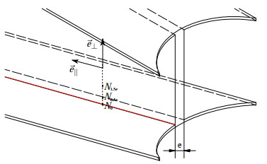Figure  2  Zone of interest (weld toe in red) for the calculation of fatigue damage for a given structure

Download: Full-Size Img

In the basis $\left(\vec{e}_{\|}, \vec{e}_{\perp}\right)$ represented in 2, the stress tensor reads:

The quantity of interest for further fatigue analysis is calculated as the maximal principal stress at % node N_0.5 with an extrapolation factor of 1.12 to account for the weld toe concentration:

where a is a constant depending on the quality of the welding process.

The quantity σ₁ is non linear against the differents stress components, obtaining error bound indicators is possible but more difficult. One can linearize this quantity of interest to compute error bounds, use quantity of interest dependent techniques or make an hypothesis on the direction of the maximal principal stress. In this paper a direction is assumed for the maximal principal as providing a σ₁ specific technique is out of the scope of this paper. This direction is assumed by expert knowledge given the geometry and the loads on the structure.

3   Computing fatigue damage from the timeseries of stress

Before defining a new strategy to propagate bounds obtained on the quantity of interest toward the fatigue damage, it is necessary to elaborate on the method to compute the fatigue damage. The method that is used in this paper follows recommended practices from Veritas (2010). Given a time series of stress obtained with the finite element method, the rainflow counting algorithm proposed in Matsuishi & Endo (1968) is used to identify stress cycles Δσ within the signal. Interested readers may refer to Veritas (2010) for an in depth explaination of rainflow counting.

A number of cycles before failure can be assigned to each Δσ using an SN curve given by standards Veritas (2010). As shown in Figure 3, the SN curve is probabilistic as the weld toe properties have intrisic variability.

Figure  3  Stress to Number of cycles curves (SN-curves)-Parameters from the D-curve for a detail in seawater with cathodic protection in Veritas (2010)

Download: Full-Size Img

4   Propagating bounds on stress toward fatigue damage

Using discretization error estimators through (15) or (16), a FEM solution S(u_h) and an interval [S⁻, S⁺] may be obtained at each timestamp $t_k\left(k \in \left[\kern-0.15em\left[ {1, n_{t s}} \right]\kern-0.15em\right]\right)$ of the time series. It is significantly different from state of the art fatigue analysis for which a single value of stress is known. Propagating bounds on stress to the damage is not a trivial task. Taking into account rainflow counting and SN-curves, damage is sensitive to the range of fluctuation and the mean stress. We focus here on the range of fluctuation. Our main concern is the range of fluctuation considering that the more (respectively the less) a signal oscillates, the larger (respectively the smaller) the total damage. The more the mean value of the stress the more the total damage. We do not consider this issue that is easier to solve: we can compute the damage with the highest value of the mean value for the stress computation without bounds and for the two signals presented in the following. Based on this hypothesis, we propose to build two signals passing within each interval delimitated by bounds:

• one maximizing damage and thus presenting maximum oscillation

• one minimizing damage and thus presenting minimal oscillations.

Signal minimizing damage  Let the signal minimizing damage be the one passing for each time stamps t_k at the point within [S⁻(t_k), S⁺(t_k)] which is the closest to the one selected for t_k−1. For t₀, we select this point as the boundary S⁻(t₀) or (S⁺t₀) closest to the first interval [S⁻(t > t₀), S⁺(t > t₀)] guaranteed to be above or below the interval[S⁻(t₀), S⁺(t₀)]. An algorithm that allows building such signal is given in Algorithm 1.

An example of such signal is shown in Figure 4(b). The signal remains constant if the value selected at t_k−1 lies in [S⁻(t_k), S⁺(t_k)] which is necessary to minimise damage. Otherwise, it will pass by either S⁻(t_k) or S⁺(t_k). Note that it is not formally proved that this signal minimizes oscilation, yet it seems to be validated by observation.

Figure  4  Signals maximizing and minizing fatigue damage

Download: Full-Size Img

Signal maximizing damage  Two signals are proposed to build the signal maximizing damage. First, we propose to use the signal successively oscillating between S⁻ and S⁺ during the time series. An algorithm that allows building such signal is given in Algorithm 2. Such signal is plotted in Figure 4(a). Note that this signal is rather unrealistic as the position of the exact solution within [S⁻, S⁺] should not vary drastically between two successive timestamps. Second, we propose to use the signal passing in each interval at the point furthest from signals mean over the whole time frame. An algorithm that allows building such signal is given in Algorithm 3. Such signal is plotted in Figure 4(b).

5   Numerical assessment: example of an offshore wind substation

5.1   Description of the structure

The substation is a critical component of an offshore wind farm as it gathers electrical power from wind turbines and exports it to shore through a single cable. Therefore, assessing accurately its structural reliability is paramount. Let us consider an offshore wind substation designed by Chantiers de l'Atlantique. The monopile layout is represented in Figure 5 and supports a 2 500 metric ton (mT) topside that is represented in Figure 1. We consider that this structure is deployed by 30 m water depth at SEM-REV test site close to Le Croisic in France. The structure is considered to be made of steel with standard material properties: density ρ = 7 800 kg/m³, Young modulus E = 210 GPa, and Poisson coefficient ν = 0.3. A single sea state modeled as a JONSWAP spectrum is simulated as a unidirectional superimposition of 50 airy waves with random phases. The topside being symmetrical and the arm being more sollicitated by waves coming from $\vec{e}_x$ than from $\vec{e}_y$ , waves propagation according to $\vec{e}_x$ is selected. The most probable sea state at the deployment site according to Ducrozet et al. (2017) is chosen: H_s = 2 m, T_p=8.5 s. We consider the fatigue failure under dynamical wave loads of the weld toe between the monopile and an arm aligned with wave propagation (see Figure 5). A two scale approach is used. First, a monopile mechanical problem is solved using dynamical beam theory to obtain loads close to the studied arm. Then a quasistatic local lower flange mechanical problem allows computing local stress a the studied weld toe (see Figure 5). The discretization error is only measured on the local mechanical problem to avoid the use of a dynamical discretization error estimator Waeytens et al. (2012) that is not available in the homemade FEM code used in this paper.

Figure  5  Offshore wind substation layout (Unit: mm)

Download: Full-Size Img

Monopile mechanical problem  First, only the monopile structure of the offshore substation (see Figure 6) is modeled. Wave loads are computed through Morison equa‐tion (Sarpkava, 1986) according to the stochastic model‐ling in Schoefs (2008); Schoefs & Boukinda (2010) and following recommended practices from Veritas (2014). The structure is considered to be fully fixed to the ground on the one end and supports a 2 500 mT inertia on the oth‐er end. The structure is modeled using dynamical beam theory. The resulting discretized mechanical problem is:

Figure  6  Monopile mechanical problem layout

Download: Full-Size Img

where U contains 2D nodal displacements, $\underline{\underline M}$ contains inertia coefficients including the topside weight, $\underline{\underline K}$ is the stiffness matrix and F(t) is the wave load on the structure. The structure is discretized into 100 element which is a compromise between a small discretization error and a good condition number of the matrix $\underline{\underline M}$ .

The mechanical problem is solved for a 3 h sea state with a time discretization of T_p/20 = 0.425 s using ode15 s in MATLAB®. The quantity of interest is σ₁₁ at the closest node to the lower flange of the studied arm (see Figure 5) that governs fatigue computation.

Lower flange mechanical problem  Second, the fatigue failure of the weld toe represented in Figure 5 is studied. In particular the point of the weld toe that is the closest to the beam web is selected as it is suspected to concentrate stress and be subjected to fatigue. For this problem σ_⊥=σ₁₁, σ_‖=σ_yy and τ_‖=σ_1y. Let us assume that σ_⊥>>σ_‖, τ_‖. It implicates:

Also, the hypothesis of 2D plane stress is made for the flange that is only subjected to loads from the monopile on the one end and is maintained fixed by the topside of the substation on the other end. As the mechanical problem is symetrical both in terms of loads and geometry, only a single symetric part of the flange is modeled. The resulting mechanical problem is represented in Figure 7. Recommended practices from Veritas (2010) suggest using a mesh size close to the zone of computation of the quantity of interest that is equal to the flange thickness that is 40 mm according to Figure 5. In order to reduce discretization error of both forward and adjoint problems at fixed computational cost, h-adaptivity Díez & Calderón (2007) is used. The resulting heterogenous mesh is shown in Figure 8 in which the mesh size close to the zone of computation of the quantity of interest is 11 mm.

Figure  7  Lower flange mechanical problem

Download: Full-Size Img

Figure  8  Mesh used for the lower flange mechanical problem

Download: Full-Size Img

5.2   Results and discussion

The method to compute bounds on the local stress σ₁ and propagate discretization error bounds toward fatigue damage is assessed on the offshore wind substation presented in 5.1. Two discretization error estimators are tested: one based on a stress smoothing technique (ZZ), one based on the error in constitutive relation and a flux free technique allowing the construction of an admissible stress field Parés et al. (2006) (ECR+FF).

5.2.1   Using ZZ error estimator

A 3 h time series of the finite element solution of σ₁ is obtained together with discretization error bounds using the ZZ estimator. A 20 s snippet of the time series is shown in Figure 9(a). The error intervals are very thin using that discretization error estimator so that the bounds cannot be seen without zooming (Figure 9(b)).

Figure  9  20 s snippet of the discretization error bounds time series obtained with the ZZ estimator

Download: Full-Size Img

Once again, note that the ZZ error estimator provides error bounds that are not guaranteed. While they can be good indicators, bounds propagated toward fatigue damage or the probability of failure are therefore not guaranteed either. Then, the signals both minizing and maximizing damage are built and the fatigue damage is computed for each of them together with the probability of failure (due to SN curve uncertainty) obtained by extrapolating the 3 h time series to 20 years of deployment. Results are given in Table 1. Two signals maximizing damage are tested: one passing the furthest from the 3 h mean of the finite element solution (Upp. bound in Table 1), one oscillating between upper and lower bound (Max. oscil. upp. bound. in Table 1). As the error interval on σ₁ is very thin, the interval is also thin on the 3 h fatigue damage and on the probability of failure. The upper bounds are fairly close using both methods. However, the upper bound using the signal passing the furthest from the 3 h mean of the FE solution is slightly greather than the upper bound using the other signal maximizing damage. It is probably because the signal oscillating between lower and upper bound is not guaranteed to pass the furthest from the 3 h mean at each turning point. Even though this signal generates a lot of cycles of small amplitude, those cycles do not have a significant contribution to the fatigue damage.

5.2.2   Using ECR+FF error estimator

A 3 h timeseries of discretization error bounds using the ERC+FF technique is also obtained. A 20 s snippet of that time series is plotted in Figure 10. First, the error intervals seem larger than with the ZZ estimator. Note that error bounds obtained with ECR+FF are guaranteed which make them more qualitative than error bounds obtain with ZZ.

Figure  10  20 s snippet of the discretization error bounds time series obtained with the ECR+FF estimator

Download: Full-Size Img

The error bounds on the fatigue damage and the probability of failure are given in Table 2. We can notice also that bounds using ZZ error estimators are included in the intervals obtained with ECR+FF estimators. While error bounds are large at turning points, the order of magnitude of the fatigue damage seems guaranteed by the error indicators. However, the error interval on the probability of failure is very large. If a smaller interval on the probability of failure was needed, turning points far from signals mean would need remeshing as only turning points are used by rainflow counting and as a quasi-static framework is used. In a dynamical framework, the remeshing strategy would have to be more sophisticated as the precision at turning points depends also on the precision at previous time stamps. Also, the upper bound using the signal passing the furthest from the 3 h average is greater than the one obtained with the signal oscillating between lower and upper bounds. The error bounds being larger at turning points, the multitude of low amplitude cycles generated by the signal oscillating between lower and upper bounds creates less damage than a signal passing the furthest from the 3 h average at turning points. It seems to indicate that the signal passing in each interval the furthest from the 3h average is a greater majorizer of damage than the signal oscillating between lower and upper bounds.

6   Conclusion

A novel approach allowing to tackle discretization error in the damage assessment of offshore structures is introduced in this paper. By using a discretization error estimator, it is possible to obtain a time series of discretization error bounds for each sea state of the scatter diagram at the deployment site. We propose a method to propagate these error bounds to obtain bounds on the fatigue damage and the probability of failure of the structure. One signal minoring damage while passing within error bounds at each time stamps is proposed. Two signals majorizing damage are proposed. The hypothesis on which these signals are built is that the more (respectively the less) a signal oscillates, the greater (respectively the smaller) the damage. While not being discussed, this hypothesis conforms with stress cycles identification through rainflow counting and SN curves. The first signal passes the furthest from the mean of the finite element solution. The second signal oscillates between lower and upper bounds at successive time stamps. The proposed method is assessed in a quasistatic framework on a beam flange of an offshore wind substation. Two estimators of the discretization error are tested. The first estimator uses a stress smoothing technique. It is available in some industrial FEM code but it is not guaranteed to give an upper bound on the discretization error. The second estimator is based on the error in constitutive relation. It is not available in industrial FEM codes but it provides a guaranteed upper bound on the discretization error. Results show that the ZZ estimator is not conservative and the second estimator should be implemented in industial codes.

This method is implemented and illustrated for the fatigue assessment of a weld toe of an Offshore Wind SubStation. Results show that the signal passing the furthest from the mean of the signal seem to give a greater upper bound on damage than the other signal maximizing damage. It is therefore recommended to use the signal passing in each interval the furthest from the mean of the signal to compute an upper bound on the fatigue damage. It should be noted that it is not proved formally that the two signals proposed to respectively minimize and maximize fatigue damage allow obtaining guaranteed error bounds on the damage. Yet, it seems to be validated by experience for both error estimators.

The direction of the maximal principal stress was assumed in order to compute error bounds on this quantity of interest. Future works should focus on either linearizing maximal principal stress with regards to the displacement field or providing a specific method to obtain guaranteed error bounds for this quantity of interest.

This paper provides a complete framework for assessing rationally the FE error that can lead to bad decisions in the context of fatigue assessment on which relies inspection planing and digital twins of marine structures. Note that the method to propagate bounds toward damage may be used for other sources of uncertainty. For example, it allows computing the error on the local damage from a monitoring system of the nominal strain close to this point.

Appendix Algorithms