1   Introduction

With the rapid development of array signal processing technologies, beamforming, a key technology of array signal processing, plays a vital role in underwater acoustic engineering. Among the beamforming algorithms, the conventional beamforming (CBF) algorithm has been widely used in underwater acoustic signal processing because of its robustness (Zhong et al. 2016). However, because of its limitation in array apertures, the performance of the CBF algorithm in practical applications is not ideal. The sidelobe of strong targets easily covers weak targets, especially when detecting weak targets under strong interference, because CBF has a high sidelobe and low resolution.

T. C. Yang creatively applied the deconvolution model to a CBF algorithm and proposed a CBF deconvolution beamforming processing algorithm (Yang 2017; Yang 2018). The algorithm retains the advantages of the CBF robustness and ensures the resolution is similar to or better than the high-resolution algorithms (Bahr and Cattafesta 2012). In recent years, scholars have conducted research on deconvolution beamforming processing technology. The research was mainly directed toward the application of a deconvolution beamforming algorithm based on an equidistant acoustic-pressure array (Xenaki et al. 2010; Xenaki et al. 2012), uniform circular array (Tiana-Roig and Jacobsen 2013), vector array (Sun et al. 2019), and deconvolution beamforming algorithms with a space-time two-dimensional joint and near-field space two-dimensional (Mei et al. 2020). As a result, the deconvolution beamforming technology advantages of low sidelobe, high resolution, and robustness have been identified.

Inspired by the CBF deconvolution beamforming algorithm, this paper studied a deconvolved Chebyshev beamforming (Dcv-Che-BF) algorithm. Chebyshev beamforming also has robustness because of the use of amplitude weighting (Li et al. 2010; Liu et al. 2018). Compared with the CBF algorithm, the Chebyshev algorithm can obtain the narrowest mainlobe width height under the condition of a given sidelobe level (Li and Liu 2005). Therefore, the Chebyshev algorithm can effectively avoid the situation when the sidelobe level is too high to distinguish the weak signal in the process of multi-target recognition. However, the resolution of Chebyshev beamforming is limited, and it is weaker than that of the CBF algorithm, especially when the preset sidelobe level is low.

This paper combines the low sidelobe characteristics of Chebyshev beamforming with the high-resolution processing ability of deconvolution beamforming. The performance of CBF, Chebyshev beamforming, minimum variance distortionless response (MVDR), CBF deconvolution beamforming, and Dcv-Che-BF were analyzed by simulation and sea trials using a uniform linear array model. DcvChe-BF retains a performance similar to the CBF deconvolution beamforming algorithm and has a better azimuth resolution.

2   Basic principle of Dcv-Che-BF

Conventional beamforming is used to compensate for the opposite time delay of the signals received by each array element. The output of each array element is superimposed to realize the in-phase addition of the expected signals of each array element and the non-in-phase addition of noise and interference to improve the output signal to noise ratio (SNR). In this study, it is assumed that under the far-field condition, the receiving array with the number of array elements N performs direction finding. The received data of each array element is processed by beamforming. The beam output results are as follows:

where Y(t)=[y₁(t), ⋯ y_N(t)]^H is expressed as the output result of array beamforming, W(θ)=[w₁(θ), ⋯ w_N(θ)] is the beamforming weight vector, which represents the weighted value of the beamformer on the data received by different array elements, and X(t)=[x₁(t), ⋯ x_N(t)]^H is expressed as the signal received by the array. θ is the angle pointed by the beam pattern, and the spatial spectrum of direction θ beam output can be expressed by beam output power as follows:

where R_X=E[X(t)X(t)^H] represents the covariance matrix of the array received signal, the matrix dimension is N × N, and E[•] is the mathematical expectation. Changing the weight vector W(θ) can change the beam output of the array such that the core of different beamformers is to solve the weight vector W(θ).

The Chebyshev beamforming algorithm mainly relies on the properties of the Chebyshev polynomial. The expansion of the Chebyshev polynomial is used to define the weight vector W_q(θ) to achieve an equal sidelobe level under the condition of setting the mainload to sidelobe ratio. The Chebyshev polynomial (Zielinski 1986) is the solution of the differential equation as follows:

$\left(1-x^2\right) \frac{\mathrm{d}^2 T_n(x)}{\mathrm{d} x^2}-x \frac{\mathrm{d} T_n(x)}{\mathrm{d} x}+n^2 T_n(x)=0$, and its n-order polynomial is expressed as

By combining the trigonometric function identity with the Chebyshev function, the Chebyshev polynomial can be obtained to meet the following recurrence relationship:

Considering an N-element linear array with equal spacing distribution, the ideal beam pattern is a real symmetric function. Therefore, its weight is real symmetric. Assuming that n is an even number, its directivity function can be expressed as:

where φ=(πd/λ)cosθ, d is the array element spacing, λ is the signal wavelength, a_m is the weight of real symmetry, and meets a_m=a_−m(m = 1, 2, ⋯, $\frac{N}{2}$). According to Equation (5), the highest order term of the N-element array polynomial R(θ) is cos[(N − 1)φ], which is a polynomial of N − 1 order. According to the properties of the Chebyshev polynomials, if the coefficients of the polynomials are equal to N − 1 order Chebyshev polynomials, the array has the best directivity, and all sidelobe heights are uniformly controllable. The maximum value of the main beam corresponds to T_N−1(x₀), and the amplitude of the sidelobe is 1. Therefore, the mainload to sidelobe ratio of the array pattern is V=T_N−1(x₀), which can be solved as x₀ = ch($\frac{1}{N-1}$ch⁻¹V). On this basis, the calculation formula of Chebyshev (Koretz and Rafaely 2009) weighted relative weight can be further obtained as:

where N ≥ k > 1, s = 0, 1, ⋯, $\left(\begin{array}{l}p \\ q\end{array}\right)=\left(\frac{p!}{q!(p-q)!}\right)(q \leqslant p)$, I_N¹ = 1. Therefore, the Chebyshev weighted weight vector of the uniform linear array can be expressed as W_q(θ)=[w_q1(θ), ⋯ w_qk(θ), ⋯ w_qN(θ)]. In this vector, w_qk(θ)=I_N^ke^{−j2π(k−1)d cos θ/λ}/N. The azimuth spectrum P(θ) of Chebyshev beamforming can be obtained using Eq. (2):

Deconvolution is the inverse process of convolution. (Hanisch et al. 1997; Biggs and Andrews 1997). Specifically, if we know the system function and the measured system output, we can deconvolute the unknown input function. In array signal processing, the beamforming spatial spectrum output of the array can be regarded as the sum of the product of the directivity function of the array at each observation angle and the angle target intensity (Mo and Jiang 2016). Therefore, it can be expressed as the following integral form:

where P(θ) represents the beamforming spatial spectrum output of different beamforming algorithms, S(ϑ) represents the objective function, reflecting the orientation and intensity information of the target, and R(θ|ϑ) represents the array directivity function of the pointing observation angle ϑ of the array corresponding to different beamforming algorithms. In this paper, R(θ|ϑ) refers to the Chebyshev weighted array natural directivity function. If the natural directivity function R(θ|ϑ) of the array does not change with the angle that meets R(θ|ϑ)=R(θ−ϑ), then R(θ|ϑ) is called the shift-invariant in the angle domain. For a uniform linear array, the natural directivity function of Chebyshev beamforming is not shift-invariant in the angle domain; however, the shift-invariant in the cosine domain. To use the shift-invariant model deconvolution iterative processing method, the model of Formula (8) is rewritten into the cosine domain convolution model, and the expression is as follows:

R(cos θ) represents the natural directivity function of the Chebyshev weighted array according to a cosine distribution, which has spatial shift invariance. In the deconvolution algorithm, it is also called the point spread function (PSF) of the system. Eq. (9) is deduced under the conditions of no noise. However, in actual data processing, the noise will inevitably have an impact on the final results. Figure 1 shows the Chebyshev weighted array natural directivity function of an 11-element uniform linear array to illustrate the shift invariance of the uniform linear array in the cosine domain. The interval of array elements is half-wavelength. The target signal is a 1 kHz single frequency signal, and the SNR is set to 25 dB.

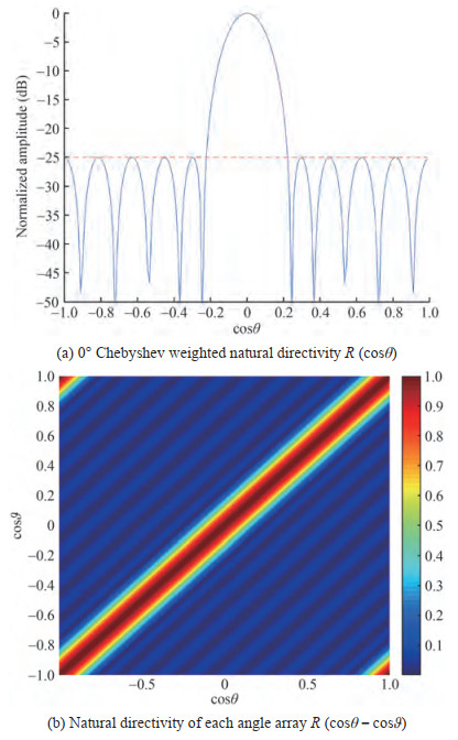Figure  1  Dcv-Che-BF PSF function

Download: Full-Size Img

As shown in Figure 1, the directivity function of the uniform linear array at different angles is the circumferential shift of the natural directivity function, so it is invariant in the cosine domain.

There are many deconvolution beamforming algorithms, including non-negative least squares (NNLS) (Chu and Yang 2013), a deconvolution approach for the mapping of acoustic source (DAMAS) algorithm (Dougherty 2005; Brooks and Humphreys 2006), and the Richardson Lucy (RL) algorithm (Richardson 1972; Blahut 2004). The RL algorithm has a better processing effect in an environment of low SNR (Ehrenfried and Koop 2006). Therefore, the RL algorithm was selected for deconvolution processing. The distribution of the signal in all directions is obtained by the RL iterative formula, which is a high-resolution signal azimuth estimation result S(cos ϑ). The specific iterative formula is shown in the following formula:

where r is the number of iterations. With the increase in the number of iterations, the result of deconvolution beamforming S(cos ϑ) gradually converges with the objective function (Hansen et al. 1999); however, the increase in the number of iterations requires more computation. Therefore, the number of iterations needs to be selected according to the actual demand. According to relevant literature, when the number of iterations is greater than 500, the performance improvement of CBF linear array deconvolution processing is very limited (Liu and Jia 2008). Therefore, this paper mainly uses 500 iterations for deconvolution processing, which can be used as the output of deconvolution beamforming to obtain a narrower mainlobe and lower sidelobe.

3   Simulation analysis

First, the performance of Chebyshev beamforming with different preset sidelobe levels was compared and analyzed under different output SNR. Note that the output SNR in this paper is equal to the input SNR plus array gain. Suppose the array is a 2-element acoustic-pressure uniform linear array. The array element space is half-wave, and the signal is a 1 kHz single frequency signal. The incoming wave direction is 0°, and the noise field is isotropic. Figure 2(a) and Figure 2(b) show the spatial spectrum results of Chebyshev beamforming and the other two methods when the output SNR is 20 dB and 7 dB.

Figure  2  Chebyshev beamforming spatial spectrum output under different SNR

Download: Full-Size Img

As shown in Figure 2(a), when the output SNR is high and the preset sidelobe level is greater than the noise background level, the lower the preset sidelobe level, the lower the actual beam output sidelobe level. However, as shown by the yellow, purple, and green dotted lines in Figure 2(b), when the output SNR is low, the sidelobe level of Chebyshev beamforming with different preset sidelobe levels does not change significantly. Therefore, the performance of Dcv-Che-BF is not better with a lower preset sidelobe level in the presence of noise. More specifically, when the output SNR is low, although the lower preset sidelobe level is adopted, the sidelobe level of the Chebyshev beamforming is still high because of the noise background level.

Several simulation experiments were conducted to further illustrate the performance of Dcv-Che-BF. The spatial spectrum results of CBF, MVDR, RL-CBF deconvolution, and Dcv-Che-BF under the conditions of Figure 2(a) are shown in Figure 3.

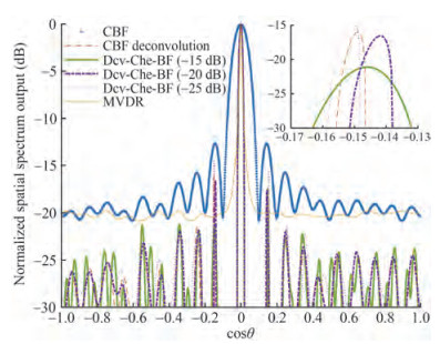Figure  3  Comparison results for a single target

Download: Full-Size Img

As shown in Figure 3, compared with conventional methods, deconvolution methods can significantly reduce the mainlobe width and sidelobe level. MVDR has the same resolution as the deconvolution methods. However, its performance is usually degraded in the actual data processing because it is sensitive to location errors. Notably, there are interesting facts identified in Figure 3. The sidelobe level of Dcv-Che-BF with a high preset sidelobe level (−15 dB) was less than that with the low preset sidelobe level (−20 dB, −25 dB), which has a totally different trend from Chebyshev beamforming.

To further explain this phenomenon, we vary the preset sidelobe level to analyze how this affects the performance of the Dcv-Che-BF under the above conditions.

As shown in Figure 4, the red dotted curve is the Chebyshev beamforming result. The blue curve is the PSF with preset sidelobe level, and the black curve is the CBF result. Deconvolution processing has the characteristic that if the actual beam output is more similar to the PSF, the deconvolution performance will be better. As shown in Figure 4(a) and Figure 4(b), the mainlobes of the Chebyshev beamforming with different preset sidelobe levels match with their corresponding PSF completely. However, it is obvious that the sidelobes of the red and blue curves in Figure 4(a) are more similar than those in Figure 4(b). The sidelobe level of PSF with the lower preset sidelobe level (−20 dB) was less than the background noise level in Figure 4(b), which affects the performance of Dcv-Che-BF. Therefore, the performance of Dcv-Che-BF was not necessarily better with a lower preset sidelobe level in the presence of noise; however, it was much better when the preset side lobe level matched the SNR of the signal. In other words, the Dcv-Che-BF method can achieve a lower sidelobe level when the preset sidelobe level was slightly greater than the noise background level.

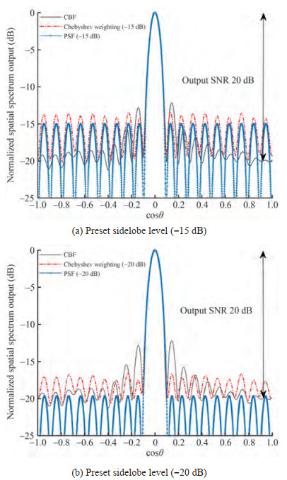Figure  4  Chebyshev beamforming spatial spectrum output with different preset sidelobe levels

Download: Full-Size Img

Several simulation experiments were conducted to verify the effectiveness of the proposed method.

Note that the SNR below is the input SNR. As shown in Figure 5, the mainload to sidelobe ratio of Chebyshev beamforming is determined by its preset sidelobe ratio. However, the trend of Dcv-Che-BF's mainload to sidelobe ratio is more complex. In the case of low SNR, the mainload to sidelobe ratio of Dcv-Che-BF is mainly limited by the noise background level but much higher than that of the conventional methods. In the case of medium SNR (5‒15 dB), the mainload to sidelobe ratio of Dcv-Che-BF with a high preset sidelobe level (−15 dB) was greater than that with a low preset sidelobe level (− 20 dB, − 25 dB), which is the same to the above conclusion. At high SNR, the mainload to sidelobe ratio of both the conventional and deconvolved methods is extremely low.

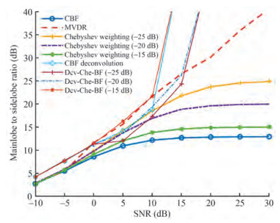Figure  5  Mainlobe to sidelobe ratios under different SNR

Download: Full-Size Img

To further illustrate the resolution of the Dcv-Che-BF methods, a simulation was considered in which there were two equal intensity targets. Suppose the first target is under the conditions of Figure 2(a). The signal of the other target is a 500 Hz single frequency signal. The resolution of the above method with different preset sidelobe levels is compared and analyzed in Figure 6.

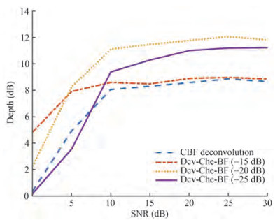Figure  6  Resolution of four deconvolution methods

Download: Full-Size Img

Note that the depth in this paper represents the depth between the trough and peak of the two targets. Therefore, the deeper the depth, the better the resolution. The depth gradually increases with the increase in SNR. At an SNR of 0 dB, the depth of Dcv-Che-BF (−15 dB) was the greatest, followed by −20 dB and then −25 dB. The depth of Dcv-Che-BF (−20 dB) exceeds the Dcv-Che-BF (−15 dB) mainload to sidelobe ratio after 5 dB, which further verifies the Dcv-Che-BF method can achieve better resolution capability when the preset sidelobe level is slightly higher than the noise background level.

Next, we varied the array elements to analyze how this affects the performance of the proposed method. Suppose the SNR is 20 dB, and the other conditions are the same as in Figure 5. The mainlobe width of the above methods under different array elements is shown in Figure 7.

Figure  7  Mainlobe width under the condition of different array elements

Download: Full-Size Img

As shown in the Chebyshev beamforming in Figure 7, the higher the preset sidelobe level, the narrower the mainlobe width, which is consistent with the theory. Dcv-Che-BF also has a narrower mainlobe width when the preset sidelobe level is greater. The mainlobe of the above methods all decreases with increasing array elements.

4   Data processing

To further evaluate the performance of the proposed method in practical applications, we analyzed the sea trial data from a towed array with different methods. The experiment was performed in the southern oceans of Sanya. The data were collected using a uniform linear array consisting of 32 elements with 0.25 m spacing. During the experiment, there were some sailing targets and other trial ships passing by on the sea surface. The strong interference around 0.95 in the cosine domain was actually the interference of the tugboat itself. The interferences around −0.8 and 0.85 in the cosine domain were two near targets. The interference around −0.07 in the cosine domain was a weak target. There were also some broadband pulse signals transmitted by other trial ships, which were reflected by the bright spots in Figure 8. The signal processing frequency band was from 1 500 Hz to 3 000 Hz. The CBF, MVDR, Chebyshev beamforming (− 25 dB), CBF deconvolution and DcvChe-BF with different preset sidelobe levels (−25 dB, − 20 dB, and −15 dB) were compared and analyzed, as shown in Figure 8.

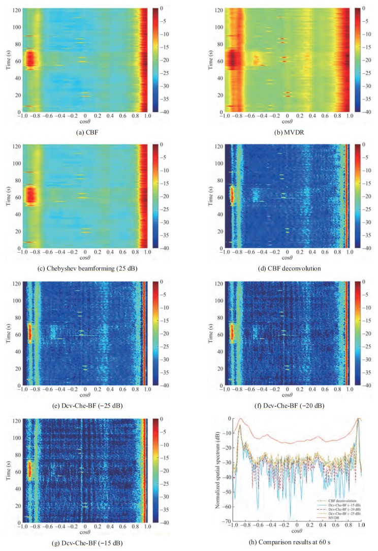Figure  8  Comparison results for the sea trial data

Download: Full-Size Img

As shown in Figure 8, the deconvolved beamforming methods can obtain a lower sidelobe level and better target resolution than the conventional methods. The performance of Dcv-Che-BF was different with the different preset sidelobe levels. As shown in Figure 8(h), although the sidelobes level of the above methods fluctuates wildly, the sidelobe level of Dcv-Che-BF(−15 dB) is the lowest. Therefore, in actual data processing, better data processing performance can be obtained by reasonably setting the sidelobe, which has also been verified in the above simulation.

5   Conclusions

Combined with the Chebyshev beamforming method, this paper introduces the deconvolution model and proposes a Dcv-Che-BF algorithm. On this basis, the influence of a preset sidelobe level on the performance of Dcv-Che-BF was further analyzed. The performance of Dcv-Che-BF was not necessarily better with a lower preset sidelobe level; however, it was much better when the preset sidelobe level was slightly greater than the noise background level. Computer simulations and sea trials results compared with CBF, Chebyshev, MVDR, CBF deconvolution, and Dcv-Che-BF has a narrower mainlobe width, lower sidelobe, and better azimuth resolution, especially in multi-target detection.