1   Introduction

Underwater cyber-physical system (UCPS) is a new complex system with high efficiency communication and effective control. It is widely used in various underwater engineering and research fields, such as resource protection, ocean environment monitoring, and early warning system of natural disaster (Gong et al. 2020; Lin et al. 2019; Wang et al. 2015). In order to support these applications, the data acquisition of underwater environment becomes a primary task to be solved. To handle this problem, internet of underwater things (IoUT), as the core components of UCPS, has attracted the interest of researches, which has advantages of low cost, rapid deployment, and self-organization (Cashmore et al. 2018; Li et al. 2019; Yan et al. 2020a).

Different from ground environment, the underwater environment has many special characteristics, which poses a substantial challenge to the underwater data acquisition. Firstly, the robustness of networks is more demanding since IoUT is a sparse network. To improve the network robustness, a common method is to improve network connectivity. However, a good connectivity can increase the energy consumption of network, which leads to shorten network lifetime. Secondly, the power of nodes in IoUT is difficult to recharge since the nodes are powered by batteries (Lin et al. 2016; Yan et al. 2021a, 2021b). Thirdly, the high-frequency radio waves are strongly absorbed in underwater environment, which cannot used in underwater scenario. Till now, the acoustic wave as the only available signal for underwater communication, but the transmission rate of acoustic wave is 1.5×10³ m/s, which is much slower than radio wave (Li et al. 2016b; Su et al. 2019; Yan et al. 2020b). Due to these challenges, the data collection schemes proposed for terrestrial sensor network are no longer suitable for IoUT.

Up to now, underwater data collection schemes can be divided into two categories: data collection by multi-hop transmission and data collection by autonomous underwater vehicle (AUV). To be specific, multi-hop transmission mainly transmits the data to the receiver (or sink node) on the water surface through a series of routing mechanisms. However, the nodes that near to the receiver consume energy quickly. Thereby, there is an imbalance of energy consumption in multi-hop transmission, which is easy to lead to the emergence of energy voids (Ren et al. 2016). For instance, Xie et al. (2006) firstly designed a vector-based forwarding (VBF) protocol, which can provide robust, scalable and energy-efficient routing. Besides that, a power-aware data collection algorithm was developed (Dhurandher et al. 2009). However, these literature were not suitable for sparse networks due to substantial energy consumed by this protocol via flooding. To reduce energy consumption, Wu et al. (2021) provided a Hierarchical Adaptive Energy-efficient Clustering Routing (HAECR) strategy to prolong the network lifetime. In Ali et al. (2014), a novel routing strategy named Layer by layer Angle-based flooding (L2-ABF) was provided under the constraints of movement of nodes, delays and energy consumption. Inspired by Xie et al. (2006), an adaptive hop-by-hop vector-based forwarding routing (AHH-VBF) protocol was designed (Yu et al. 2015). Some other multi-hop transmission based data collection schemes were presented (Jin et al. 2017; Wei et al. 2013). Although these schemes can achieve energy efficient, the robustness of the network is not considered. For the second category, the data collection task is completed by assistance of AUV. In Khan and Cho (2014; 2016), multiple AUVs assisted data collection method was proposed. Besides that, Han et al. (2019) developed a prediction-based delay optimization data collection method to solve the issue of data collection delay. In Duan et al. (2020), the value of information was utilized as a metric to measure the quality of information. In view of this, a reliable hierarchical information collection system was constructed for data collection. In addition, Cai et al. (2019) applied the mobile edge elements into data collection algorithm, whose results were helpful to solve the problem of unbalanced energy consumption. In Han et al. (2018), a stratification-based data collection algorithm was proposed for underwater data collection with constraints of water delamination and limited-energy. Although these algorithms help to improve the energy efficient, how to improve the robustness of network has not been well studied. We notice that topology is a good way to balance network connectivity and energy consumption. Referring to Shames and Summers (2015), we found that the rigid characteristics of the network are closely related to its algebraic properties. In Luo et al. (2018), the potential-game based optimally rigid topology control algorithm was proposed to improve the network performance. The rigid graph based topology optimization algorithm was employed to balance the trade-off between energy consumption and network connectivity in Yan et al. (2016). Although the works in Luo et al. (2018) and Yan et al. (2016) demonstrate a good trade-off between energy consumption and connectivity maintenance, the relationship between topology optimization and routing strategy has not been studied. With regards to limited-energy and network connectivity, how to adopt the topology optimization technology to balance the trade-off between the energy efficient and network connectivity for routing algorithm is still an open issue.

With the assumption of the data is collected by data collector, some path planning schemes have been proposed for AUV. For instance, the path planning problem of multiple robots was studied for data collection in Bhadauria et al. (2011). In McMahon and Plaku (2017), the sampling-based motion planning were incorporated into constraint-based solvers to achieve autonomous data collection. Nevertheless, the methods in Bhadauria et al. (2011) and McMahon and Plaku (2017) only consider the effect of geographical location on AUV data collection, the validity of the data is not considered. Since the data generated by the nodes has associated values that decay over time, it is necessary to consider the value information of the collected data. Based on this, the timeliness of the data was used to plan the path of AUV in Gjanci et al. (2018), Liu et al. (2022), then maximize the effective value of the total data collection. Our previous work (Yan et al., 2018) developed a dynamic value-based path planning method for AUV to maximize the value of information. However, the obstacle avoidance is not addressed. With consideration of geographical location of nodes, timeliness of the data and obstacle, how to design the path planning and tracking strategy of AUV is another problem to be solved.

With these problems in hand, an AUV-assisted energy-efficient data collection scheme is proposed in this paper. Two phases data acquisition algorithm is designed, i. e., routing algorithm design for sensor nodes and path planing for AUV. In the first phase, the optimal rigid graph was incorporated into dynamic routing algorithm for sensor nodes to transmit the data to data collector. Of note, the proposed method can balance the trade-off between the energy consumption and the network robustness. Subsequently, the Q-learning based AUV path planning strategy is developed in the second phase to periodically accesses the data collector and periodically resurfaces the water to unload the collected data to the control center. In particular, the main contributions of this paper are as follows:

1) Routing algorithm design for sensor nodes. The potential game based optimal rigid graph is designed to balance the trade-off between the energy consumption and network connectivity, and then a Q-learning based dynamic routing algorithm is provided for sensor nodes to relay the collected data to data collector. Compared with the existing works (Li et al. 2016a; Yan et al. 2018), the routing algorithm in this paper can prolong the network lifetime and improve the robustness of network.

2) Path planning and tracking for AUV. A Q-learning based path planning algorithm is developed for AUV to guide the movement of AUV, and then a proportional-integral-derivative (PID) based tracking algorithm is proposed to track the desired path. Compared with the existing work (Han et al. 2017), the path planning algorithm in this paper can improve the information value of the total data collection with a time limit and avoid the influence of environmental obstacles.

2   System model and problem formulation

2.1   System model

As depicted in Figure 1, a network including sensor nodes, data collectors and AUV is designed for data collection.

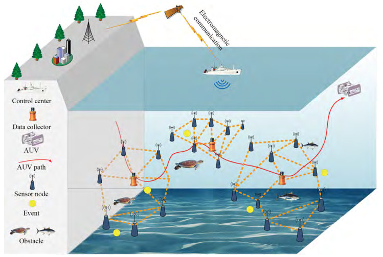Figure  1  Description of the network architecture, where an AUV is employed to retrieve data from multiple data collectors

Download: Full-Size Img

• Sensor Nodes. The role of sensor nodes is to perform underwater monitoring tasks, whose clocks are synchronized and the coordinates are accurately known. It should be emphasized that, sensor nodes can move passively due to the effect of current.

• Data Collectors. Data collectors are static nodes, whose function is to gather data from sensor nodes through some routing mechanisms. Particularly, the locations of data collectors are fixed with the anchor wire constraints.

• AUV. An AUV is deployed to visit data collectors, through which the data can be retrieved by high speed visible light communications. Meanwhile, AUV periodically surfaces to offload the retrieved data to control center via high speed radio communications. Without loss of generality, we assume that the batteries equipped on AUV are sufficient.

Similar to Yan et al. (2018), the underwater monitoring area is divided into M subareas. It is noted that N sensor nodes and one data collector are deployed in each subarea. For an arbitrary subarea, sensor nodes collect data from the surrounding environment and send the collected data to data collector through single-hop or multi-hop communication. Without loss of generality, we assume that a set E of events E₁, …, E_|E| occur in the underwater monitoring area, where |E| is the total number of events. When sensor node i∈{1, …, N} has sensed an event E_k at time t_{k, i}, the value of information (VoI) C_{Ek, i} for the sensed data on event E_k can be acquired by sensor i, where 1≤k≤|E|. Specially, the VoI C_{Ek, i} at time t is defined as

where $F_{E_k} \in \mathcal{R}^{+}$ and e^{−(t−t_{k, i})} denote the event importance and timeliness of E_k, respectively. 0≤β_k≤1 represents the information weight, whose role is to balance the trade-off between importance and timeliness. It is noted that, the event importance can be designed and modified according to the monitoring levels. Meanwhile, the event timeliness is a monotonically decreasing function, which is to captures the temporal decay of the sensed data. This is intuitive as later retrieve of a data segment can lead to higher losses.

Different from the terrestrial networks, the sensor nodes in IoUT move passively since the effect of current. Based on this, a meandering current mobility model (Xia et al. 2017) is utilized to describe the movement of sensor nodes. Accordingly, the movement of sensor node i∈{1, …, N} can be updated as

where $\left(x_i, y_i, z_i\right) \in \mathcal{R}^3$ denotes the position of sensor node i, ψ(x_i, y_i, t)=−tanh$\left[\frac{y_i-B(t) \sin \left(\kappa\left(x_i-c t\right)\right)}{\sqrt{1+\kappa^2 B^2(t) \cos ^2\left(\kappa\left(x_i-c t\right)\right)}}\right]$, $\rho \in \mathcal{R}^{+}$ is an iteration scalar, $z_{\text {fix }, i} \in \mathcal{R}$ is the predefined fixed depth of sensor node i, ϑ_i∈$\mathcal{R}$ follows White Gaussian noise (WGN), κ∈$\mathcal{R}$ is the number of meanders in the unit length, and c∈$\mathcal{R}$ denotes the phase speed. Particularly, B(t)=A+ϵ cos(ωt) modulates the width of meanders, wherein A∈$\mathcal{R}$ resolves the average meander width, ϵ∈$\mathcal{R}$ represents the amplitude of the modulation, and ω∈$\mathcal{R}$ denotes its frequency. In a data gathering cycle, we assume that the change of water current is not frequent and the sensor nodes cannot move out of the predefined subareas.

Referring to Sehgal et al. (2011), the energy consumption when transmitting one packet over distance d can be calculated as

where d is the transmission distance between one sensor node and its next-hop node, SL∈$\mathcal{R}^{+}$ denotes the sonar source level, $\vec{l}$ denotes the transmission loss range, α represents the absorption coefficient in dB/km, TL denotes the transmission loss, and T_tx is the transmission time of a single packet.

It is noted that, the body-fixed reference frame (BRF) and inertial reference frame (IRF) are adopted to describe the AUV dynamics. Due to the intrinsic stability of rolling and pitching of open-frame vehicles (Caccia and Veruggio 2000; Kim et al. 2016), this paper presents a simplified model including four degrees of freedom (4-DOF), i.e., neglecting pitch and roll motions. Based on this, the dynamics of AUV is formulated as

where u, v, and w denote the linear velocities in surge, sway and heave, respectively. r denotes the angle velocity in yaw. Besides, m_u, m_v, and m_w denote the masses in surge, sway and heave, respectively. I_r is the moment of the inertia in yaw. F_u, F_v and F_w are the exerted forces in surge, sway and heave, respectively. T_r is the exerted torque in yaw and W is the buoyancy force in heave. k_u, k_v, k_w, and k_r are the linear damping scales in surge, sway, heave and yaw, respectively. k_u^*u|u|, k_v^*v|v|, k_w^*w|w| and k_r^*r|r| are the quadratic damping constants in surge, sway, heave and yaw, respectively. In view of (4), the kinematics of AUV can be described as

where x, y, and z are the positions on X, Y and Z axes, respectively. φ denotes the angle in yaw.

2.2   Problem formulation

Problem 1 (Routing strategy design for sensor nodes) Since the complexity of underwater environment, such as coral reefs and fish stocks, it affects data transmission and requires higher robustness to networks. Meanwhile, the battery power installed on underwater sensor node is limited and cannot be recharged. In order to avoid the energy holes and prolong the network lifetime, the optimal rigid graph is incorporated into dynamic routing algorithm to relay the data from sensor nodes to data collector. This problem is reduced to optimize the routing selection of sensor nodes with the consideration of energy holes and network robustness.

Problem 2 (Path planning and tracking for AUV) In mobile IoUT, data collectors gather data from sensor nodes, but the collected data is decaying with time. To maximize the VoI of data delivered to control center, we aim to design a Q-learning based path planning strategy for AUV to find the desired path, which can avoid environmental obstacles effectively. Of note, the AUV dynamics are highly complex, and the exact dynamic parameters of AUV are not easy to acquire due to the influence of ocean currents. To solve this issue, a model-free tracking tracking controller is sought to be provided, such that AUV can accurately track the desired path.

3   Energy-efficient data collection approach

In this section, the energy-efficient data collection approach is developed. As shown in Figure 2, the approach is divided into two phases, i.e., 1) routing strategy for sensor nodes; 2) path planning and tracking for AUV. The detailed process of the two phases is described below.

Figure  2  Framework of energy-efficient data collection approach

Download: Full-Size Img

3.1   Routing strategy for sensor nodes

Without loss of generality, the routing strategy of sensor node is divided into two stages, i. e., optimal rigid graph design and dynamic routing algorithm design. In the following, the routing strategy for sensor nodes is given.

3.1.1   Optimal rigid graph design

For ease of description, an arbitrary subarea S₁ is taken as an example. Without loss of generality, subarea S₁ can be modelled as a graph $\mathcal{G}(\mathcal{V}, \mathcal{E})$, in which $\mathcal{V}$={1, 2, …, N, N+1} is the set of sensor nodes and data collector in subarea S₁, and $\mathcal{E}=\{(i, j) \in \mathcal{V} \times \mathcal{V}: i \neq j\}$ is the edge set. Of note, each edge in the graph is expressed by a different pair of vertices (i, j). If any vertex pair (i, j) of graph $\mathcal{G}(\mathcal{V}, \mathcal{E})$ satisfies $\forall(i, j) \in \mathcal{E} \Rightarrow(j, i) \in \mathcal{E}$, then graph $\mathcal{G}(\mathcal{V}, \mathcal{E})$ is called an undirected graph, otherwise it is called directed graph. Especially, graph $\mathcal{G}(\mathcal{V}, \mathcal{E})$ is called rigid graph if vertex is removed does not destroy the stability of graph. Otherwise, it is called a flexible graph. It is noted that, it is called minimum rigid graph if the rigid graph becomes flexible when any an edge is removed from rigid graph. For a clearer description, examples of a flexible graph, a rigid graph, and a minimum rigid graph are given in Figure 3. Accordingly, the following definition and lemma are given.

Figure  3  Example of flexible and rigid graphs

Download: Full-Size Img

Definition 1 (Zhang et al. 2015) Defining $\mathit{\boldsymbol{\mathcal{R}}}_{(\mathcal{G})} \in \mathcal{R}^{|\mathcal{E}| \times| 3\mathcal{V} \mid}$ is the rigidity matrix of a graph $\mathcal{G}(\mathcal{V}, \mathcal{E})$ with N+1 vertices in 3D space. The graph is called a infinitesimally rigid graph if and only if the rank of $\mathit{\boldsymbol{\mathcal{R}}}_{(\mathcal{G})}$ is 3(N+1)−6, i.e, rank($\mathit{\boldsymbol{\mathcal{R}}}_{(G}$)=3(N+1)−6.

Lemma 1 (Luo et al. 2013) $\mathcal{G}_i(i=1, 2, \cdots, N+1)$ is a minimum rigid graph, which composes of node i and its neighborhood. $\mathcal{G}(\mathcal{V}, \mathcal{E})=\bigcup_{i=1, \cdots, N+1} \mathcal{G}_i$. Denote the generated optimal rigid graph as $\mathcal{G}_{\text {opr }}\left(\mathcal{V}, \mathcal{E}_{\text {opr }}\right)$. Then, the following statements hold: a) $e \notin \mathcal{E}_{\text {opr }}$, if $e=(j, k) \in \mathcal{E}$, $j, k \in \mathcal{G}_i$, and $e \notin \mathcal{G}_i$; b) The optimal rigid graph $\mathcal{G}_{\text {opr }}\left(\mathcal{V}, \mathcal{E}_{\text {opr }}\right)$ can be obtained by deleting those edges satisfying a).

The aim of this section is to balance the trade-off between the network stability and energy consumption by optimizing network topology. Of note, each node (i. e., data collector or sensor node) in the network is independent and affects each other. Based on this, the game theory is introduced to optimize the network. Without loss of generality, a strategy game consists of three elements, i.e., Player $\mathcal{I}$, Strategic Space $\mathcal{A}$, and Utility Function $\mathcal{U}$. Thus, the strategy game is expressed as $\mathit{\Gamma }\{\mathcal{I}, \mathcal{A}, \mathcal{U}\}$. In the following, the three elements of strategy game are introduced in detail: 1) Player $\mathcal{I}$∈{1, 2, …, i, …, N+1}, where N+1 is the total number of players in game; 2) Strategic Space $\mathcal{A}: \mathcal{A}=\mathit{\Pi }_{i \in \mathcal{I}} \mathcal{A}_i$ is the set of all possible combinations of policies for all players to choose. a=(a_i, a_−i) is the strategic of all players, where $a_i \in \mathcal{A}_i$ is the strategy selection by player i and a_−i is the strategic selection of players other than player i; 3) Utility Function $\mathcal{U}: \mathcal{A} \longrightarrow \mathbb{R}$ for $i \in \mathcal{I}$ is mappings. Based on this, the following definitions are given.

Definition 2 (Nash Equilibrium (NE)) (Chen et al. 2019; Lee et al. 2018) The strategy a^*=(a_i^*, a_−i^*) is said to be Nash Equilibrium, if $\mathcal{U}_i\left(a_i^*, a_{-i}^*\right) \geqslant \mathcal{U}_i\left(a_i, a_{-i}^*\right)$ always holds, where a_i^* is the best strategy of player i to other players, a_−i^* is the best strategy of players other than player i.

Definition 3 (Ordinal Potential-Game (OPG) and Ordinal Potential Function (OPF)) (Chen et al. 2019; Lee et al. 2018) For game $\mathit{\Gamma }\{\mathcal{I}, \mathcal{A}, \mathcal{U}\}$, if there exist a function $\mathcal{U}(a)\mathcal{A} \rightarrow \mathbb{R}$, $\forall i \in \mathcal{I}$, $\forall a_{-i} \in \mathcal{A}_{-i}$, for $\forall a_i^a \in \mathcal{A}_i$ and $a_i^b \in \mathcal{A}_i$, the following equation holds

Then, the game $\mathit{\Gamma }\{\mathcal{I}, \mathcal{A}, \mathcal{U}\}$ is called OPG, and the function U(a) is called OPF of the game $\mathit{\Gamma }\{\mathcal{I}, \mathcal{A}, \mathcal{U}\}$.

Based on the above definitions, the following two aspects are considered to construct the utility function.

1) Energy consumption of network: Similar to Yan et al. (2018), the relative energy consumption is adopted to describe the energy consumption. Define the required energy at time t as RE(t), which is calculated by (3). The available energy at time t is denoted as AE(t). Based on this, the relative energy consumption of sensor node i is defined as $E_i(t)=\frac{\operatorname{AE}_i(t)}{\operatorname{RE}_i(t)}$. For nodes i and j, i≠j and i, j∈{1, 2, …, N+1}, we assume that the node i sends the data packet to its neighbor node j, and the available energy of nodes i and j is greater than the required energy. Then, the energy-based model is described as

where N_i is the neighborhood node set of node i.

Without loss of generality, we assume that the same parameters (i.e., SL and α) are used in the monitoring area. Then, one has RE_i(t)=RE_j(t)=RE_ij(t). Thus, (7) can be rearranged as $f_1=\max \sum_i \sum_{j \in \mathcal{N}_i} W_{i j}(t)$, where W_ij(t) = (AE_i(t) + AE_j(t))/RE_ij(t) is the weight between nodes i and j. In view of this, the rigidity matrix $\mathit{\boldsymbol{\mathcal{R}}}_{(\mathcal{G})}$ can be defined a

where p_i=[p_i¹, p_i², p_i³]^T and p_j=[p_j¹, p_j², p_j³]^T are the coordinates of nodes i and j, respectively. Of note, each row $\left[0 \cdots 0 \frac{\left(\boldsymbol{p}_i^{\mathrm{T}}-\boldsymbol{p}_j^{\mathrm{T}}\right) W_{i j}}{\left\|\boldsymbol{p}_i^{\mathrm{T}}-\boldsymbol{p}_j^{\mathrm{T}}\right\|} \cdots \frac{\left(\boldsymbol{p}_j^{\mathrm{T}}-\boldsymbol{p}_i^{\mathrm{T}}\right) W_{i j}}{\left\|\boldsymbol{p}_j^{\mathrm{T}}-\boldsymbol{p}_i^{\mathrm{T}}\right\|} 0 \cdots 0\right]$ corresponds to one edge $(i, j) \in \mathcal{E}$.

2) Stability of network: To ensure the stability of the network, definition 1 must be satisfied. In view of this, the following function is defined

Subsequently, the vertex rigidity gramian $\boldsymbol{X}_{(\mathcal{G})}$ is given to reflect the algebraic quality of network, i.e., $\boldsymbol{X}_{(\mathcal{G}}=\mathit{\boldsymbol{\mathcal{R}}}_{(\mathcal{G})}^{\mathrm{T}} \mathit{\boldsymbol{\mathcal{R}}}_{(\mathcal{G})} \in\mathit{\boldsymbol{\mathcal{R}}}^{|3 \mathcal{V}| \times|3 \mathcal{V}|}$. It is noticed that the trace of the vertex rigidity gramian is the sum of the eigenvalues of the rigidity matrix. Therefore, the following optimization problem is given

Therefore, the utility function of game $\mathit{\Gamma }\{\mathcal{I}, \mathcal{A}, \mathcal{U}\}$ can be constructed as

where $\boldsymbol{X}_{\left(\mathcal{G}, a_i\right)}$ is the vertex rigidity gramian with the strategy a_i.

In view of (11) and Lemma 1, the potential game based optimal rigid graph can be generated, and the corresponding pseudo codes are described in Algorithm 1. It should be emphasized that the Algorithm 1 contains two principles, i. e., 1) keeping the network is a minimum rigid graph, and 2) maximizing the trace of the vertex rigidity gramian.

3.1.2   Dynamic routing algorithm design

With the generated optimal rigid graph in the Section 3.1.1, the communication topology of network can be obtained. To transmit the data from sensor nodes to data collector, the Q-learning based dynamic routing algorithm is designed. As we know, Q-learning is a learning algorithm, the agent (i.e., sensor node) select the optimal action through the interact with an external environment. The learning process of network can be modeled as a Markov decision process with limited state and action space, it can be denoted as M = (S, A, R), where S is the set of nodes (i.e., state set), A is the set of optional node (i.e., action set), and R is the reward function. Of note, each state in this section has N+1 optional action. To evaluate the performance of actions, the reward function R(s_l¹, a_l¹) at lth episode step is designed as

where $\mathcal{R}_{{\rm{max}}}$ is the maximum bonus value, which implies that the next state is the data collector. $-\mathcal{R}_{{\rm{max}}}$ is a negative value, indicating that there is no communication between the two states. d_{l, l+1}=||p_l−p_l+1|| is the distance between the nodes l and l+1. Besides that, s_l¹, s_l+1¹ and a_l¹ are the current state, the next state and the current action, respectively.

According to R(s_l¹, a_l¹), the Q function can be updated by the following equation, i.e.,

where α is the learning rate, γ∈[0, 1) is the discount factor, and a_l+1¹ denotes the next action.

Therefore, the Q-learning based dynamic routing algorithm is given in Algorithm 2. It is noted that the sensor node selects the node with the maximum Q value as the next hop to forward data based on the Q table. The sensor node can transmit the data to data collector by shortest distance. Even if one transmission path is interrupted, the sensor node can transmit data to data collector successful. Therefore, it can guarantee to prolong network lifetime and improve the network reliability.

3.2   AUV path planning strategy

With the routing strategy for sensor nodes in Section 3.1, the data collector can collect the data from sensor nodes successfully. Define a binary variable k_{k, i} with i∈{1, …, N}, k_{k, i}=1 if sensor i sense the event E_k, otherwise k_{k, i}=0. Similarly, a binary variable l_{j, i} with j∈{1, …, M} is defined to express whether data collector j can obtain the VoI of sensor i, i.e., l_{j, i}=1 if the data collector j can receive the VoI of sensor i, otherwise l_{j, i}=0. Accordingly, the VoI of sensor i and VoI of data collector j from sensors can be calculated as

With the above discussions, we employ the AUV to collect the information from the data collectors. AUV access the data collector periodically and unload the collected data to the control center. The access period time of AUV is defined as T. It is noted that the time of vertical movement is important for data collection at the next data collection cycle. Based on this, we assume that the depth of the data collector is h and the vertical velocity of AUV is v, then the time that AUV vertical movement to data collector is $t_{\text {vertical }}=\frac{h}{v}$. Therefore, the data collection time of AUV is updated as T=T−2t_vertical. Besides that, we assume that the communication range of data collector is the maximum accessible distance under the fixed transmission power of AUV. Each data collector broadcasts a data packet to AUV via acoustic communication, which contains the position information of the data collectors and the VoI of the collected events. Accordingly, the income function of data collector j is designed as

where t∈[0, T], D_j(t) is the distance between current position of AUV and data collector j. The purpose of subtraction of D_j(t) is to reduce the distance of access. $\bar{\alpha} \in \mathcal{R}^{+}$ is a scalar. In view of (16), the income function of AUV can be expressed as

where t_in is the time that AUV start to collect data.

Based on (17), one knows that AUV dynamically select the data collector with the largest income function as the destination at the next time. Due to the obstacles of the underwater environment, the Q-learning based path planning strategy is adopted to plan the optimal path of AUV for data collection. At the beginning, the AUV submerge to the depth of the data collector with the largest income function. Then, the current position of AUV is set as the initial state and the data collector with the largest income function is set as the destination. Of note, the area is uniformly divided into $\mathcal{M}=n \times n$ lattices, in which each lattice corresponds to a state and its corresponding Q value is zero. Based on this, there are $\mathcal{M}$ states. Different from Section 3.1, each state in this section has four optional action, i.e., action set includes moving toward east, west, north and south. To evaluate the performance of actions, the reward function RA(s_l², a_l²) is defined as

where $\mathcal{R}_{A, \max }$ is a maximum positive value. In addition, s_l², s_l+1² and a_l² are the current state, the next state and the current action of AUV, respectively.

Based on this, the Q function is given as

where α₁ is the learning rate, γ₁ is the discount factor, and a_l+1² is the next action of AUV.

Similarly, the pseudo codes of Q-learning based path planning strategy of AUV is presented in Algorithm 3. It is noted that the information value of the data collector, the effect of geographical location and environment obstacles are all considered.

According to Algorithm 3, the dynamic path planing of AUV can be obtained, i.e., the desired trajectory of AUV is acquired. Since the accurately dynamic parameters of AUV is difficult to obtain, the model-free tracking controller is developed to drive the AUV to track the desired trajectory. Considering that the PID controller is simplicity, easy implementation, excellent performance and meeting the demand of tracking, the PID tracking controller is employed in this paper for tracking. Without loss of generality, the trajectory of AUV is defined as X_AUV=[x, y, z]^T and the desired trajectory of AUV is denoted as X_r=[x_r, y_r, z_r]^T. Thus, the position tracking error is computed as e=X_r−X_AUV. Define F=[F_u, F_v, F_w]^T. To ensure X_AUV→X_r within a limited time interval, the PID tracking controller is designed as

where K_p is proportional gain, K_I is integral gain and K_d is derivative gain. Besides that, Δe(t)=e(t)−e(t−1) denotes tracking velocity error.

Obviously, the PID tracking controller does not require model information of AUV. In view of (Zhao and Guo 2017), the PID tracking controller can guarantee that the AUV can accurately track the desired trajectory by adjusting the parameters of K_p, K_I and K_d.

4   Performance analysis

Theorem 1 The potential game based optimal rigid graph is 3-connected. The average node degree of each node is 6.

Proof According to Algorithm 1, the generated graph is the minimum rigid graph. From the properties of the minimum rigid graph, it can be seen that each node in the optimal rigid graph has at least three communicating neighbor nodes for rigidity requirement. Thereby, the potential game based optimal rigid graph is 3-connected.

Clearly, the number of edges of optimal rigid graph is $\mathcal{E}=3(N+1)−6$. Referring to (Yan et al. 2018), we know that the sum of the degree of all nodes is twice the number of edges. Thus, the degree of all nodes is computed as 2(3(N+1)−6). Define the average degree of each node is AD, then one has $\mathrm{AD}=\frac{2(3(N+1)-6)}{N+1}$. It is noted that the average degree of each node converges to 6 with the increasing of the nodes number, i.e., lim_N+1→∞AD=6. Thereby, the average degree of each node is 6.

Theorem 2 Under the condition of the minimum rigidity, the optimal rigid graph in this paper has the shortest communication link and the largest weight sum of the energy balance under the condition of maximizing algebraic characteristic.

Proof Take subarea R_i as an example. According to definition 1, we know that the number of edges of the minimum rigid graph is 3(N+1)−6. The proposed optimal rigid graph can ensure that the network has the least communication links under the condition of ensuring connectivity and stability.

Clearly, the energy consumption of the sensor nodes is used to receive data and transmit data. According to (3), one knows that the energy consumed by transmitting data is mainly related to distance between receiver and transmitter. We assume that the number of data packets is received by each node is same, then the energy consumption problem of sensor nodes is mainly determined by the energy consumed by transmitting data.

According to Algorithm 1, the weight of energy balance is maximized with maximizing the weight of rigid matrix. Thus, the transmission energy consumption of the sensor node is minimized. Due to the transmission energy consumption is mainly related to the transmission distance, the communication link of sensor node is minimized. Clearly, this proof also suitable for other subarea.

Theorem 3 The game model $\mathit{\Gamma }\{\mathcal{I}, \mathcal{A}, \mathcal{U}\}$ for optimal rigid graph is an OPG. The function $U(a): \vec{A} \longrightarrow \mathbb{R}$ is an OPF of $\mathit{\Gamma }\{\mathcal{I}, \mathcal{A}, \mathcal{U}\}$.

Proof The ordinal potential function is defined as U(a_i, a_−i $\sum_{i \in \mathcal{V}} \mathcal{U}\left(a_i, a_{-i}\right)$ and let $\Delta \mathcal{U}_i=\mathcal{U}_i\left(a_i^b, a_{-i}\right)-\mathcal{U}_i\left(a_i^a, a_{-i}\right)$, where a_i^a and ab i are two different strategies of node i. Then, the difference between the utility functions of the two different strategies can be calculated as

Then, the signs of ΔU and $\Delta \mathcal{U}_i$ are analyzed as follows, i.e.,

If h_i(a_i^b, a_−i)=h_i(a_i^a, a_−i)=1 holds, then one has

According to Definition 2 and Definition 3, one can obtained that the game model $\mathit{\Gamma }\{\mathcal{I}, \mathcal{A}, \mathcal{U}\}$ for optimal rigid graph is an OPG. The function $U(a): \mathcal{A} \rightarrow \mathbb{R}$ is an OPF of $\mathit{\Gamma }\{\mathcal{I}, \mathcal{A}, \mathcal{U}\}$. The proof is completed.

Theorem 4 Q-learning-based dynamic routing algorithms do not have data loops in the process of data fusion.

Proof According to (12), the reward function is set to the maximum reward value R_max when the next state is the data collector, the reward function is set to a negative value −R_max when the two nodes are not communication, and the reward function is set to −d_{i, j} when the nodes are communication but the next state is not the data collector. According to (13), we know that the Q value is higher when the communication link is close to the data collector. Therefore, the consistency of the transmission direction can be guaranteed.

5   Simulation results

In this section, simulation results are presented to prove the effectiveness of the proposed algorithm. Without loss of generality, a monitoring area of size of 250 m×250 m×250 m is divided into M subareas, N sensor nodes and one data collector are deployed in each subarea. In each subarea, the data is collected by sensor nodes from surrounding environment. Subsequently, sensor node sends data to the data collector by single-hop or multi-hop manner. Of note, the number of sensor nodes and subareas are mainly determined by monitoring performance requirements. The more the number of sensor nodes and subareas, the higher the accuracy of data collection, but the higher the monitoring cost. Especially, the parameters used in simulation are given in Table 1. Accordingly, the initial deployment of the network is shown in Figure 4.

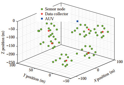Figure  4  Initial deployment of network

Download: Full-Size Img

5.1   Simulation for routing path of sensor nodes

The results of routing path of sensor nodes are analyzed in this section. Since the routing path of each subarea is similar, only the results of arbitrary subarea S₁ are investigated, i.e., the results of other subarea are omitted in this paper.

To verify the performance of dynamic routing algorithm, two cases are considered: 1) the static underwater environment; and 2) the dynamic underwater environment. Under case 1, the nodes in network are stationary. Based on this, the routing path of sensor nodes in this paper is shown in Figure 5(a). Correspondingly, the residual energy of sensor nodes under the method in this paper is described in Figure 5(b). In Li et al. (2016a), the sensor nodes forward the data to data collector through the neighborhood nodes, which is not the optimal communication topology. Under the same assumption, the routing path and residual energy of sensor nodes are shown in Figure 5(c) and Figure 5(d), respectively. In addition, a local routing decision strategy was proposed to complete data collection from sensor nodes in Yan et al. (2018). Accordingly, the routing path and residual energy of sensor nodes are shown in Figure 5(e) and Figure 5(f), respectively. From Figures 5(a)-(d), one knows that the method in this paper can prolong the lifetime of network and the robustness of network can be guaranteed. Referring to (Shames and Summers 2015), one knows that the rigid graph with the larger eigenvalues of determinant has better algebraic properties and the stability of the network is improved accordingly. Inspired by this, the trace of X_(G) under the methods in (Yan et al. 2018) and this paper isshown in Figure 6(a). From Figure 6(a), Figures 5(a)-(b), Figures 5(e)-(f), we can see that the methods in (Yan et al. 2018) and this paper are both effective for data collection and the stability of network is improved in this paper.

Figure  5  Results for routing path under case 1

Download: Full-Size Img

Figure  6  Algebraic properties

Download: Full-Size Img

In case 2, the sensor nodes can be moved under the influence of ocean current. Based on this, the routing path and residual energy of sensor nodes under the method in this paper are shown in Figure 7(a) and Figure 7(b), respectively. Under the same assumption, the routing path and residual energy of sensor nodes under the method in Li et al. (2016a) are shown in Figure 7(c) and Figure 7(d), respectively. Correspondingly, the routing path and residual energy of sensor nodes under the method in Yan et al. (2018) are shown in Figure 7(e) and Figure 7(f), respectively. Besides that, the trace of X_(G) under two methods is shown in Figure 6(b). Obviously, the network lifetime can be prolonged by compare with the ones in Li et al. (2016a) and the stability of network can be improved by compare with the ones in Yan et al. (2018). Therefore, the proposed routing path method is meaningful.

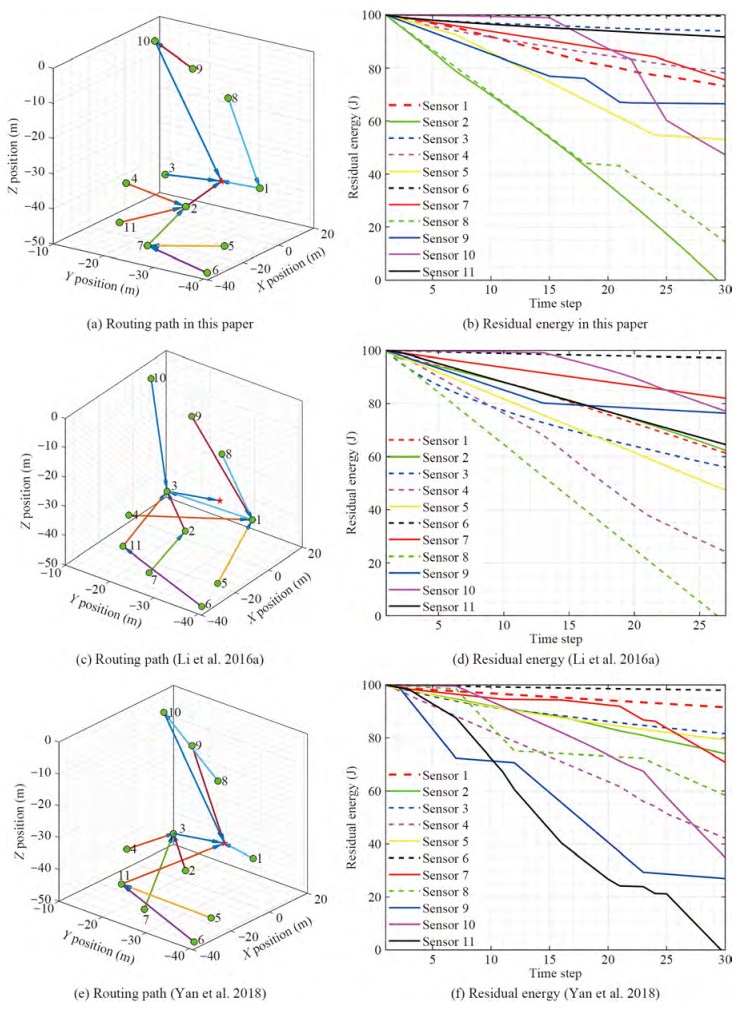Figure  7  Results for routing path under case 2

Download: Full-Size Img

5.2   Simulation for path planning and tracking of AUV

In order to verify the effective of the path planning in this paper, the VoI collected by data collectors are set as: RC₁= 0, RC₂= 2.4, RC₃= 1.8, RC₄= 3.5, RC₅= 3.8+0.3t, and RC₆= 0.05, where t∈ [0, 160]. Based on the VoI, the AUV analyzes the VoI of data collectors and path planning through Algorithm 3. Accordingly, the path planning of AUV (i.e., desired trajectory of AUV) with the method in this paper is shown in Figure 8(a). In Han et al. (2017), the traveling salesman problem (TSP) strategy was developed to plan the trajectory of AUV. Under the same assumption, the path planning of AUV with the method in Han et al. (2017) is described in Figure 8(b). From Figures 8(a)-(b), we can seen that the path planning of AUV under the method in this paper is more appropriate comparing with the method in Han et al. (2017), since the VoI of data collectors 1 and 6 are small, they do not need to be accessed by AUV. Of note, accessing valueless data collectors can increase the offload time for the collected data to the control center on the sea surface. To verify the effectiveness of the proposed algorithm, the environmental obstacles are set in paths 2 and 3, i.e., the pink area in Figure 8(c). Accordingly, the path planning of AUV from data collector 2 to data collector 3 is shown in Figure 8(c), where the optimal path of AUV is represented by red origin. Clearly, the Q-learning based AUV path planning algorithm in this paper can effectively avoid the impact of environmental obstacles.

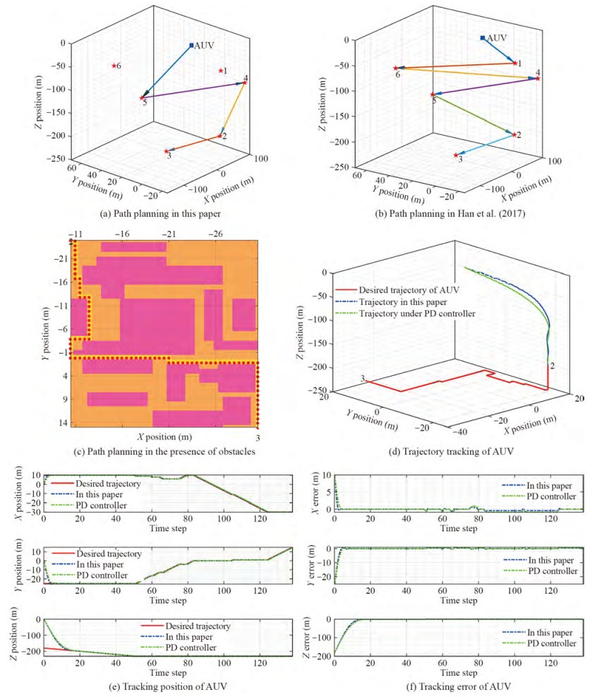Figure  8  Simulation results for path planning and trajectory tracking of AUV

Download: Full-Size Img

Based on the desired trajectory of AUV, the PID tracking controller is employed for tracking. In the simulation, we only give the part of 2→3. Based on this, the tracking trajectory with the method in this paper is shown in Figure 8(d). Correspondingly, the tracking position and tracking error are shown in Figure 8(e) and Figure 8(f), respectively. According to Thenozhi and Yu (2014), we found that the PD controller can achieve tracking but has a steady-state error, which can be reduced by introducing an integral term. Therefore, the PID controller can achieve a zero steady-state error. Based on this, the tracking trajectory, tracking position, and tracking error under the PD tracking controller are shown in Figures 8(d)-(f). Obviously, PID controller has better performance than PD controller.

6   Conclusion

With consideration of energy consumption, network robustness, and environmental obstacles, the energy-efficient data collection issue for IoUT has been studied in this paper. At the beginning, the potential game based optimal rigid graph strategy is proposed to balance the tradeoff between the energy consumption and the network stability. Based on optimal communication topology, the Q-learning dynamic routing algorithm for sensor nodes is developed to collect data from sensor node to data collector. Then, Q-learning based AUV path planning algorithm is presented for AUV to plan trajectory to collect data from data collector, through which the PID tracking controller is utilized to track desired trajectory. Finally, simulation results show that the proposed algorithm can ensure the energy efficient and network stability by compare with some existing works, and the PID tracking controller can track desired trajectory well. In the future, we will further expand the verification fields of the experimental platform.