1   Introduction

Shoreline change analysis to identify erosion trends or accretion (Ariffin et al. 2018; 2019; Selamat et al. 2019; Zulfakar et al. 2020; Mathew et al. 2020) provides critical inputs to coastal scientists, engineers, and managers. Accordingly, there must be a proper definition of shorelines to commence shoreline change analysis. A shoreline is expressed by the point where land meets water (Kraus and Rosati 1997). The boundary, however, is considered dynamic due to the forces exerted on it. These indicators are used to represent shorelines and can be divided into two types: features that can be seen on coastal images and those that are formed when a specific tidal datum intersects a coastal profile (Boak and Turner 2005). The most common technique of defining shorelines is a visual interpretation of features, also known as proxy-based shorelines, such as high-water line (HWL) shorelines. Meanwhile, shorelines that are determined by the intersection of two specific tidal datums, such as mean high-water (MHW) shorelines, are referred to as datum-based shorelines.

Proxy-based shorelines are easily accessible for long-term historical shoreline change research because they can be recognized by aerial photography and historical land-based photographs (Crowell et al. 1991). However, proxy-based shoreline identification is subject to error and is less accurate when compared to in-situ measurements. It is also hardly repeatable as it includes human interpretation and the possibility of error from image correction (Crowell et al. 1991). Using profile measurement (GPS) or LiDAR (Stockdon et al. 2002), shorelines can be assessed using a datum-based approach that does not rely on visual cues and is, therefore, more repeatable than the proxy-based approach (Moore et al. 2006). Conversely, the data gathering to derive datum-based shorelines is usually extremely chal lenging, time-consuming, and labor-intensive (Ruggiero and List 2009).

The locations of HWL shorelines are frequently more landward than the locations of MHW shorelines (Ruggiero et al. 2003). The horizontal offset between HWL and MHW shorelines, referred to as the proxy-datum bias, is primarily influenced by wave-driven water level variations and wave setup and swash oscillation, as stated by Ruggiero et al. (2003) and Moore et al. (2006). Considering the growing popularity of datum-based shoreline usage and the increasing use of LiDAR data (Stockdon et al. 2002; Zhang et al. 2002; Sallenger et al. 2003), it is critical to assess the proxy-datum bias. This integrates available historical shoreline data (proxy-based) and modern data (datum-based) in shoreline change studies.

The proxy bias is slope dependent, with low sloping beaches having a high bias value. Variations in the wave height and wavelength (period) are the most responsible for variability in bias estimates for beach slopes steeper than approximately 0.05. For beach slopes shallower than 0.05, the bias variability is primarily determined by the beach slope itself (Ruggiero and List 2009). The shoreline change rate alteration owing to the proxy-datum bias will be mainly defined by the magnitude of the shoreline change rates (Moore et al. 2006). For instance, in locations where the proxy-datum offset is slight or when the analysis period is long, the shoreline change rate shift may be negligible. However, this paper aims to evaluate the proxy-datum bias for the Kuala Nerus shoreline.

2   Study area

Kuala Nerus is a district in Terengganu, a state on Peninsular Malaysia's east coast that faces the South China Sea. Every year, the area experiences southwesterly prevailing wind (southwest monsoon) from late May to September and northeasterly prevailing wind (northeast monsoon) from November to March (Ariffin et al. 2016; Zulfakar et al. 2020). As the main tidal station for the study area, Kuala Terengganu is semi-diurnal and micro- to meso-tidal (Ariffin et al. 2018), with a mean higher high water (MHHW) of 3.92 m and mean lower low water (MLLW) of 1.88 m measured from the Peninsular Malaysia Geodetic Vertical Datum (DTGSM).

In 2008, the Sultan Mahmud Airport in Kuala Terengganu built a land reclamation to accommodate an airport runway extension (Muslim et al. 2006; Ariffin et al. 2016;2018; Zulfakar et al. 2020). The reclamation included the construction of a groin-like structure that stretches roughly 1 km toward the sea (Figure 1). The extension's nature has altered the coastal transport pattern, affecting the local environment (Ariffin et al. 2018). Downdrift erosion has been observed in the Tok Jembal and Universiti Malaysia Terengganu (UMT) areas since the project was completed (Jaharudin et al. 2019).

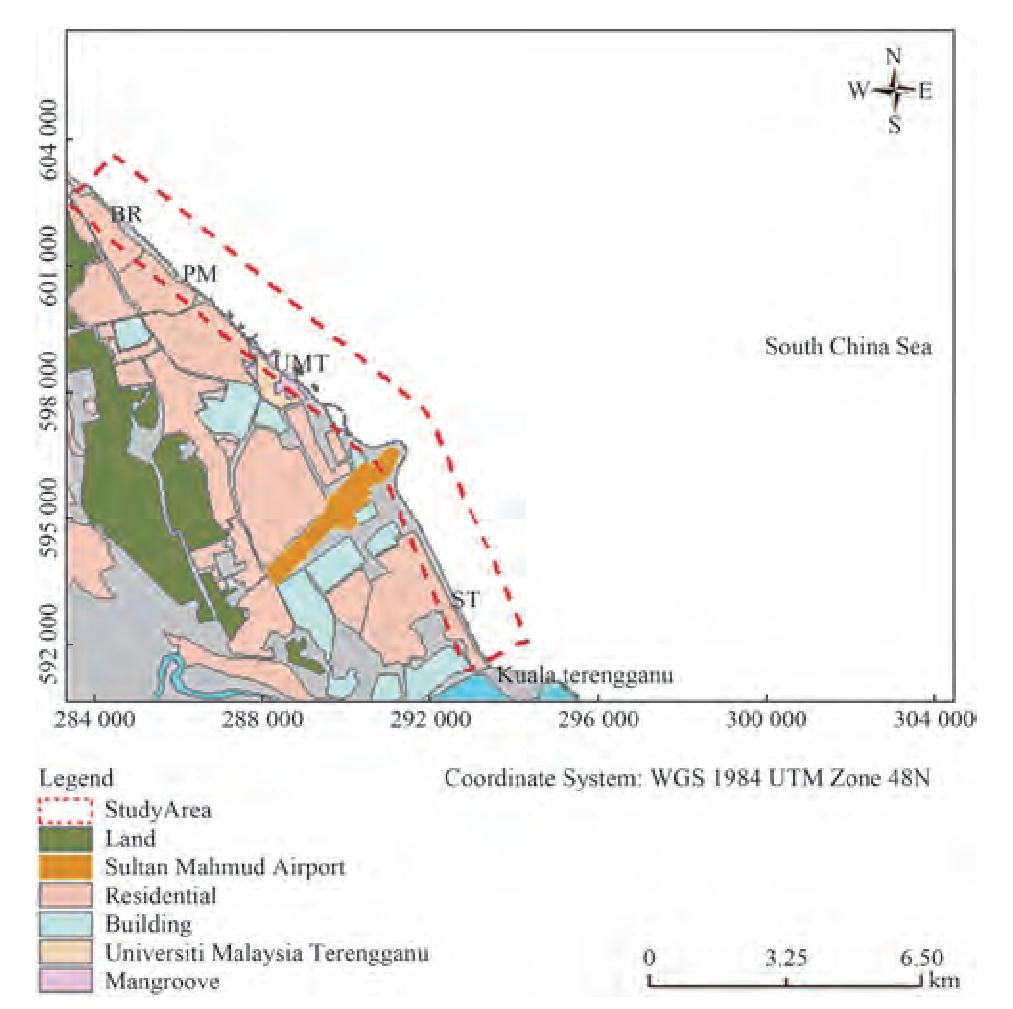Figure  1  Location of beach profiling. Batu Rakit (BR), Pengkalan Maras (PM), Universiti Malaysia Terengganu (UMT), and Seberang Takir (ST) within the study area

Download: Full-Size Img

According to a numerical study performed to examine erosion from 2010 to 2014, the average retreat within 3 km of the Sultan Mahmud Airport is 24.88 m (2012), 33.90 m (2013), and 42.93 m (2014) (Subiyanto et al. 2019). The shoreline of Kg. Pak Tuyu, 4 km north-western of Sultan Mahmud Airport, has been proclaimed as class I erosion (critical erosion) by the National Coastal Erosion Study (Department of Irrigation and Drainage, Malaysia, 2015), with a declared erosion rate of 11.8 m/yr. Because downdrift erosion was encountered in the study region, various studies have been conducted to determine the rates of retreat and progradation of the shoreline in the area. In these studies, shoreline identification was accomplished by digitizing the shoreline using a proxy (HWL shoreline) (Ariffin et al. 2018; Selamat et al. 2019; Zulfakar et al. 2020) as proxy-based shoreline indicators, such as the HWL, are typically used when data needed for a datum-based shoreline indicator are not available (Borrelli and Boothroyd 2020).

3   Available data

3.1   Measured beach profile

Beach profiles were measured 64 times along the study area shoreline from 2015 to 2020 at four locations: Batu Rakit (BR), Pengkalan Maras (PM), UMT, and Seberang Takir (ST) (Figure 2). The surveys were performed during low tide with tide information based on the tide level predicted at the Kuala Terengganu tide station, the main tidal station for the study area. The Kuala Terengganu tidal type is semi-diurnal and micro- to meso-tidal (Ariffin et al. 2018). The tide ranges from 2 m to 4 m with an MHHW of 3.92 m and MLLW of 1.88 m measured from the DTGSM. The measurement month for each location and their count are tabulated in Table 1.

The surveys incorporated the use of a theodolite, levels, and a total station model Topcon GM-50 supplied by Sky-Shine Corporation (M) Sdn. Bhd, manufactured by Topcon Corporation (Japan). Profiles were measured beginning at a recognized benchmark and ending at approximately 0.5 m water depth with an average length of 40-60 m with a horizontal resolution of approximately 1 m. The measured beach profiles were processed using Profiler 3.2 XL program (Cohen 2016) to obtain the beach slope and align the profiles with the DTGSM (Figure 2). In this study, beach profile data, i.e., the median beach slope recorded over the measurement period, were utilized as a parameter to determine the theoretical proxy-datum bias. In addition, the beach profiles were utilized in determining the measured proxy-datum bias. Beach profiling and aerial photography must be simultaneously executed to precisely measure the proxy-datum bias. However, due to the lack of consistent measurements, the comparisons in this study were made using profile measurements taken within a month period of the aerial photography.

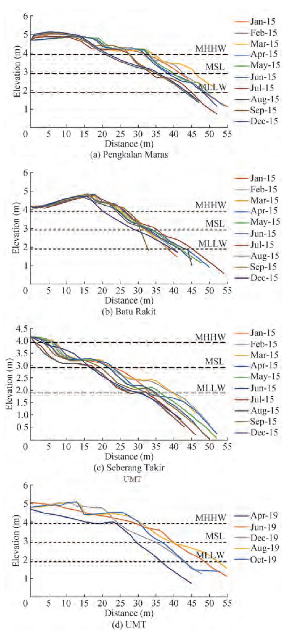Figure  2  Measured beach profiles at PM (2015), BR (2015), ST (2015), and UMT (2019). Profiles are vertically adjusted to Peninsular Malaysia Geodetic Vertical Datum (DTGSM)

Download: Full-Size Img

3.2   Aerial photographs

Aerial photographs of the study area shoreline were acquired in two separate campaigns. The first campaign was conducted at 9: 30 AM on October 1, 2018, and the flight covers UMT and PM. The second campaign was conducted at 08: 00 AM on May 21, 2019, with the coverage of UMT, PM, and BR. Aerial photographs were taken using an unmanned aerial vehicle, which is DJI's Mavic 2 Pro drone. Mavic 2 Pro has a maximum flight altitude of 500 m (Vellemu et al. 2021). A 160 m flight height was set above the ground level to obtain a wide coverage of the study area (Jayson-Quashigah et al. 2019; Mohamad et al. 2021). The survey flight lines were prepared in a third-party application called Litchi, an efficient application to plan an auto-flying drone survey. The fly settings involved were the altitude, speed, and heading of the drone. The acquisition of photographs was automatically set to one shot per second, and the flight lines covered 4.2 km of the area at every one-time flying (Figure 3), with a total of 1945 aerial photographs acquired over the study area.

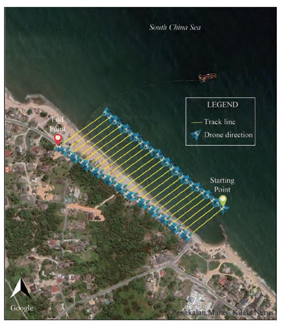Figure  3  Flight lines for the auto-fly survey that have been planned in the Litchi application

Download: Full-Size Img

The drone flying height was set at an average of 160 m above the ground level (drone home point), resulting in an aerial photo resolution of 6.5 cm/pixel (Pujianiki et al. 2020). The remote navigator only manually pilots the take-off and landing operations. The acquired aerial photographs were then processed in a software package of Agisoft PhotoScan LLC (Mancini et al. 2013) for the purpose of framing the images in the UTM 48N coordinate system. In addition, 86 randomly distributed ground control points (GCPs) were established within the survey area (Liu et al. 2018; Shoab et al. 2022). The GCP coordinates were taken using real-time kinematics for georeferencing purposes to correct the position and ground elevation of the photos by relating the image data to real features on the ground (Figure 4). The GCPs were selected based on permanent structures, i.e., buildings. The georeferencing of the aerial photographs resulted in 0.2 m absolute horizontal accuracy and 0.35 m absolute vertical accuracy.

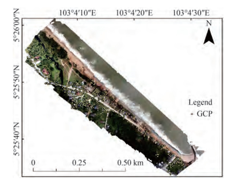Figure  4  Map of the ground control point (GCP) taken by random distribution using the real-time kinematic tool

Download: Full-Size Img

3.3   Wave data

The wave data were obtained from the European Centre for Medium-Range Weather Forecasts (ECMWF) ERA-Interim (ECMWF Reanalysis) dataset, which is available from January 1, 1979, to August 31, 2019 (https://www.ecmwf.int/). ERA-Interim is a global climate atmospheric reanalysis that integrates model data with assessments worldwide (Berrisford et al. 2009). The ERA-Interim data for the ocean wave parameter are accessible at a resolution of 1° × 1°. This research used the wave parameters at 104° E 6° N, approximately 110 km offshore of the study area.

4   Methods

4.1   Estimation of the HWL, MHW shoreline, and measured proxy-datum bias

The HWL distinguishes the landward extent of the last visible high tide and is identified by sand color alteration. It is also noticeable in aerial photographs, which are commonly displayed by a change in color or gray tone (Crowell et al. 1991). To estimate the HWL shoreline, a line marking the last visible high tide, approximated by the change in sand color, was drawn on an octorectified aerial photograph in the ArcGIS software (Figure 5).

Figure  5  HWL determination based on sand color alteration at Pengkalan Maras (PM)

Download: Full-Size Img

While the HWL shoreline is determined using visual interpretation, the MHW shoreline can be precisely and efficiently distinguished from a specific site with sufficient beach profiling data (Boak and Turner 2005). To accomplish this, an MHHW value of 3.92 m above the DTGSM datum from the Kuala Terengganu tide station was applied as the MHW to identify the horizontal distance between the start of the profile and the point where the MHW coincides with the profile (Figure 6).

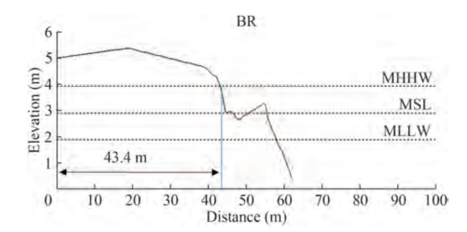Figure  6  Determination of MHW shorelines. Distance from the start of the profile to the MHW intersection

Download: Full-Size Img

Beach profiling and aerial photography must be simultaneously executed to precisely generate the measured proxy-datum bias value. Nevertheless, the comparison can only be made using profile measurements taken within a month of the aerial photography campaign due to the lack of consistent measurements. Based on the highest intertidal range of the study area beach, the daily water line delineation was assumed to be subject to a maximum uncertainty of 3 m in the delineation (Zulfakar et al. 2020). Using ArcGIS, the derived HWL and MHW shorelines were compiled in a map, and the distance between the shorelines was calculated (Figure 7).

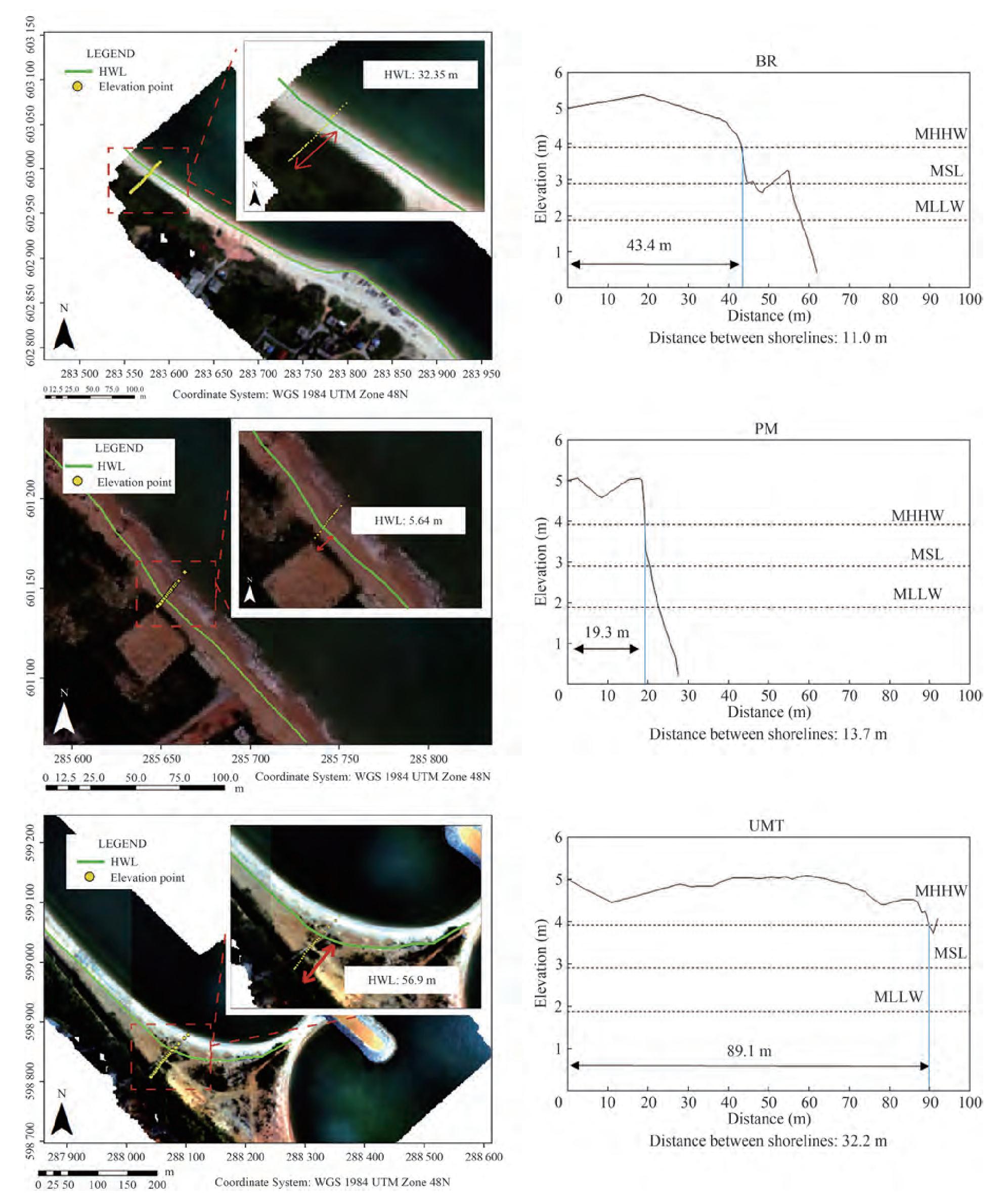Figure  7  Derived HWL and MHW shoreline compilation and determination of the distance between the two shorelines

Download: Full-Size Img

4.2   Estimation of the theoretical proxy-datum bias

Ruggiero et al. (2003) and Moore et al. (2006) established an approach for calculating the proxy-datum bias. Using an estimated total water level (TWL) model,

where Z_t is the measured tide level and R_stat is the wave runup. Using data from field experiments, Stockdon et al. (2006) developed an empirical interaction for extreme wave runup elevation that can be applied in the TWL model. The TWL relation applies to natural beaches in a variety of conditions (Ruggiero and List 2009), as follows:

where tanβ is the foreshore beach slope, H_o is the offshore wave height, L_o is the offshore wave length, given by linear theory as (g/2π) T², where g is the acceleration of gravity; and T is the wave period.

Stockdon et al. (2006) inferred that the foreshore beach slope is roughly linear in the proximity of the MHW. The proxy-datum datum bias, a horizontal offset between the HWL and MHW shorelines that can be measured cross-shore, can thus be estimated by

Eq. (2) can be rearranged as follows:

Ocean wave data from the ECMWF for the years 2009–2019 were analyzed. The variables for the above estimation were assessed by employing the procedure proposed by Ruggiero and List (2009) to guesstimate the proxy-datum bias for shoreline studies. This procedure adopted the median value from the ocean wave data while the median of the foreshore beach slope from the measured beach profiles from each location was utilized. The median wave height (0.58 m), wave period (5.6 s), and wavelength (49.5 m) values were obtained from the ocean wave data analysis, and Figures 8, 9, and 10 show the analyzed wave parameters.

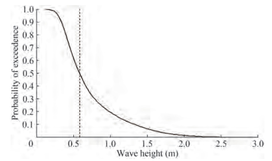Figure  8  Median wave height

Download: Full-Size Img

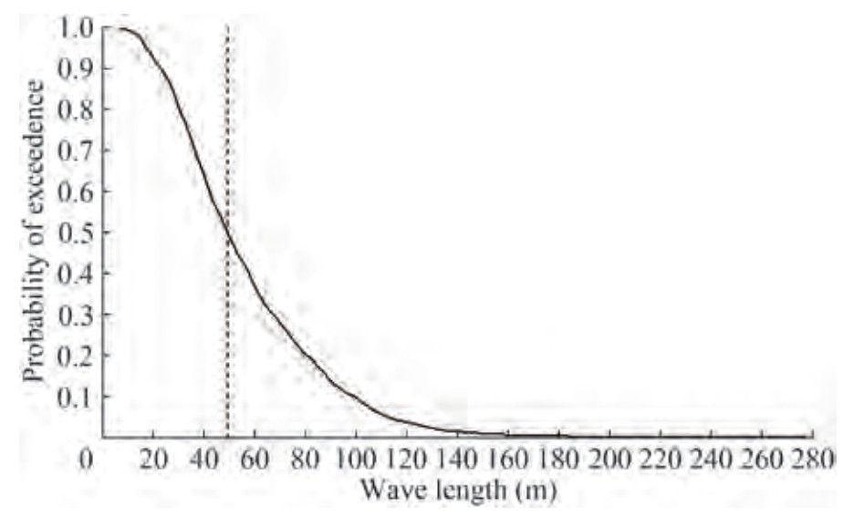Figure  9  Median wave length

Download: Full-Size Img

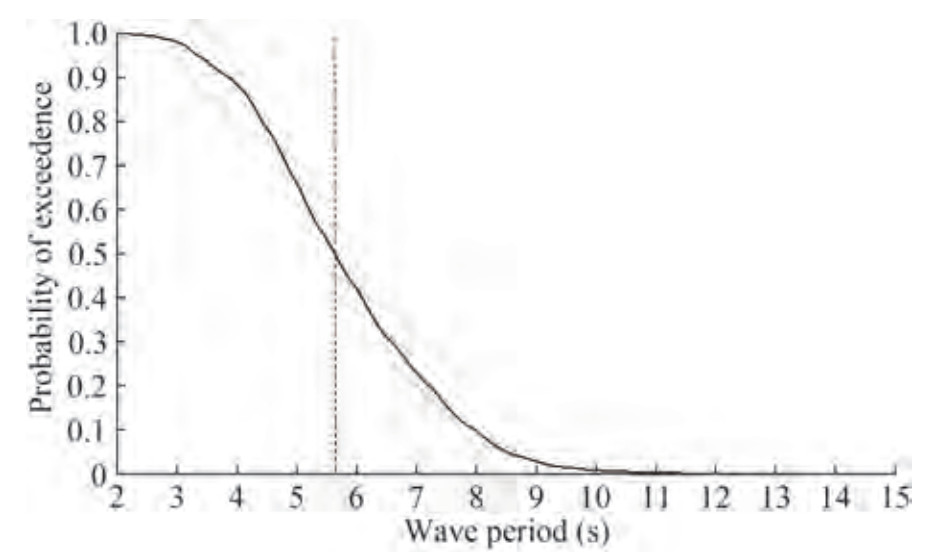Figure  10  Median wave period

Download: Full-Size Img

5   Results and discussion

In the study area, a horizontal offset exists between the proxy-based and datum-based shorelines. For steep sloping beaches (> 0.05), variations in wave height and wavelength (period) are most responsible for variabilities in bias estimates, while for beach slope shallower than 0.05, bias variability is primarily determined by the beach slope itself (Ruggiero and List 2009). In an area with a relatively high wave climate and low sloping beach, the horizontal offset can be up to 32 m (Ruggiero et al. 2003). However, this study confirms that even in a moderately steep sloping beach (> 0.05), a large horizontal offset will exist between two shorelines, as reported by Moore et al. (2006).

Table 2 summarizes the median beach slope and theoretical and measured proxy-datum bias. The measured proxy-datum bias in the study area pursues the theoretical estimation trend, i. e., increasing the bias as the beach slope decreases. Throughout the study area shoreline, the median beach slope ranges from 0.06 to 0.16, with the shallowest slope detected at UMT and the steepest slope recorded at ST. The largest offset was measured at UMT (32 m), and the distinction between the measured and theoretical values is comparable, with the most remarkable difference occurring at UMT, which has the shallowest beach slope (Figure 11).

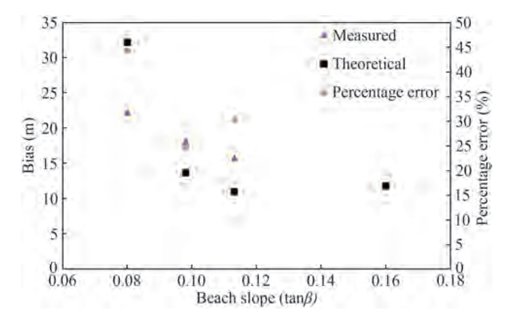Figure  11  Beach slope against the measured bias, theoretical bias, and percentage error

Download: Full-Size Img

The highest error value between the measured and theoretical biases was found at UMT (44.4%), recorded at the shallowest beach slope among the beaches in the study area. In general, the PM and BR beaches with steep slopes recorded relatively small error values. The study was conducted on a meso-tidal beach shoreline with a moderately sloping beach. While the meso-tidal area may have a relatively small tide range, other factors, such as significant wave actions, may cause the HWL (proxy-based) to be further landward than the MHW line (datum-based) due to the effects of the setup and wave runup (Liu et al. 2014). In future shoreline change studies, this type of shoreline area needs to incorporate proxy-based shoreline (historical data) and datum-based shoreline (modern data), and a theoretical one can be utilized to estimate the horizontal offset between two shorelines, with particular care on relatively mild sloping beaches.

The increased application of LiDAR data and vertically corrected digital elevation models have led to the growing popularity of datum-based shorelines. As a result, additional analysis was conducted to quantify the impact of incorporating the derived bias into shoreline change rate studies that utilize proxy-based and datum-based shorelines. Following the recommendations of Moore et al. (2006), the generated rate shift of shoreline changes is a small element of inaccuracy relative to the rates of shoreline alteration under most circumstances. However, the fast pace of shoreline changes could further result in severe errors in shoreline change rates.

The shoreline at the vicinity of Sultan Mahmud Airport experienced a progradation of 3 m in 2000. Nonetheless, the shoreline change rate shows a retreat of 24 m in 2009 and 46 m in 2010, indicating rapid shoreline changes in the study area, as documented by Muslim et al. (2006). The retreat in this area was 11.38 m in 2012 (Ariffin et al. 2018). This value is regarded as a rapid shoreline change rate, and further research on the impact of the proxy-datum bias should be performed to improve the precision in potential shoreline change rate research in the study region.

The theoretical proxy-datum bias was determined by utilizing a median value of the beach slope and wave parameters over the measurement period. Thus, the resulting bias value is representative of the median condition, but it cannot represent the beach slope seasonal variability. The research was conducted in an area with a predominantly monsoon climate, and its shoreline tends to erode and accrete in response to the monsoon condition (Ariffin et al. 2018). Thus, further research shall be performed to include intra-annual beach slope variabilities due to seasonal monsoon in determining the proxy-datum bias.

6   Conclusion

Using proxy-datum data, the researchers found a tendency toward increasing the horizontal bias as the beach slope decreases according to theoretical predictions. The study area's proxy-datum bias was the highest at UMT (32 m) and lowest at BR (11 m). This study also indicated that the theoretical estimates of the proxy-datum bias based on the TWL model produced comparable values to the measurement, with a reasonably small disparity in the bias for steep beach slopes. As the proxy-datum bias is a value that identifies the horizontal offset between the proxy-based shoreline and datum-based shoreline in any specific case, the value could be incorporated to either proxy-based shorelines by shifting the shoreline seaward or to datum-based shorelines by shifting the shoreline landward in order of the bias value (Ruggiero and List 2009). Future shoreline change rate studies in an area with meso-tidal type can benefit from the comparison between measured and theoretical proxy-datum biases.