-
Abstract
This paper proposes a risk assessment model considering danger zone, capsizing time, and evaluation time factors (DCEFM) to quantify the emergency risk of ship inflow and calculate the degree of different factors to the emergency risk of water inflow. The DCEFM model divides the water inflow risk factors into danger zone, capsizing time, and evacuation time factors. The danger zone, capsizing time, and evacuation factors are calculated on the basis of damage stability probability, the numerical simulation of water inflow, and personnel evacuation simulation, respectively. The risk of a capsizing scenario is quantified by risk loss. The functional relationship between the location of the danger zone and the probability of damage, the information of breach and the water inflow time, the inclination angle and the evacuation time, and the contribution of different factors to the risk model of ship water inflow are obtained. Results of the DCEFM show that the longitudinal position of the damaged zone and the area of the breach have the greatest impact on the risk. A simple local watertight plate adjustment in the high-risk area can improve the safety of the ship.Article Highlights• To comprehensively quantify the ship water inflow risk, a DCEFM risk assessment model is proposed.• The factors affecting ship water inflow risk are studied, and the influencing factors were determined as the danger zone, capsizing time, and evacuation time factors.• The risk assessment of a ship is carried out, and the longitudinal position of the damaged area and the breach area had the greatest impact on the risk.• A simple local watertight plate adjustment in the high-risk area can improve the safety of the ship. -
1 Introduction
With the increasing demand for ships in various countries, ship enlargement has become the trend of ship industry development. The increase in marine structures will raise the frequency of ship flooding accidents and the risk of ship flooding. The research on the risk model of ship water inflow is important for determining the factors leading to risk, analyzing the probability and consequences of risk, and improving the safety of marine structures.
Risk assessment has been applied to different fields of ships in recent years. Liwang (2012) combined the probabilistic risk assessment method with the actual needs of vessels and proposed a safety scenario determination method based on operational tasks. Prill (2016) studied the impact of ship maneuvering on ship risk. Lee (2013) conducted a numerical simulation of ship collision and grounding accidents to assess ship safety.
The frequency and consequences of ship water inflow accidents are related to multiple factors and have strong randomness (Hu et al. 2019; Zhang et al. 2020b). Ship water inflow is an inevitable stage after ship damage. Gao (2012) used Computational Fluid Dynamics (CFD) to evaluate the characteristics of cabin sloshing in the ship water entry process and simulated the forced roll motion of the ship under complete and damaged states. Larmela (2007) simulated the continuous inflow model to replicate water flow between interconnected cabins. Gao (2010; 2011) wrote an N-S solver in CFD to influence the water inflow in the house and used the solver to simulate the water inflow of the cabin to handle the coupling motion between the water inflow and the damaged ship through the dynamic grid technology. Stern (2013) summarized the application of CFD simulation technology in boats and indicated that RANS had a good simulation effect on ship heave and pitch motion. The simulation time remained to be a significant problem faced by CFD technology. This technology can accurately capture the flow field information, a powerful tool for the shipping industry to analyze the interaction between flow field and ship (Hashimoto et al. 2017; Zhang et al. 2020a; 2021).
Damage stability is an important index to measure the safety of ships after damage. The cabin damage stability calculation method has changed from a deterministic approach to a more reasonable probabilistic one (Bulian et al. 2020; Vassalos and Mujeeb-Ahmed 2021). Vassalos et al. (1997) analyzed the factors that may cause ship dumping, combined the probability and consequences of various factors, and took the obtained results as the probability of ship dumping. Matsuda (2016) conducted a quantitative safety assessment of damaged ships using numerical simulation technology from cabin damage stability. The stability analysis was simplified with the development of simulation software. Huang (2015), Lu et al. (2018), and other scholars verified that the simulation software could realize the damage stability assessment.
Casualties are indicators used to measure the consequences of risky events. The evacuation process of large ships is remarkably complex. The loss of direction under mobile platforms and panic conditions complicate the evacuation of ships compared with ordinary land buildings (Vassalos et al. 2001; Lee et al. 2004). Considering the impact of the loss scenario on the ship, assuming the evacuation of personnel when the vessel is in an emergency is necessary and reasonable (Kim et al. 2020; Wang et al. 2021).
Ship risk is inevitable, and a reasonable assessment of ship risk can improve ship safety in the design stage. This paper constructs a water inflow emergency risk assessment model (DCEFM) based on background of ship water inflow. The DCEFM decomposes the water inflow risk factors into danger zone, capsizing time, and evacuation time factors. Based on probabilistic damage stability assessment and water inflow time-domain and personnel evacuation simulations, the degree of each risk factor on the total risk is solved, and the capsizing scenario risk is quantified by risk loss. The suggestions for subdivision optimization are finally introduced in accordance with the risk loss.
2 Construction of DCEFM
Ships will encounter various risks in their life cycle, and the risks in different loss scenarios are different. The probability of death loss usually measures the risk. Jasionowski and Vassalos (2006) studied this aspect and proposed a risk model.
Risk model:
$${{\mathop{\rm Risk}\nolimits} _{{\rm{PLL}}}} \equiv E(N) \equiv \sum\limits_{i = 1}^{{N_{\max }}} {{F_N}} (i)$$ (1) where Nmax is total number of people on board.
FN curve is given by the following formula:
$${F_N}(N) = \sum\limits_{i = 1}^{{N_{\max }}} f {r_N}(i)$$ (2) frN (N) is calculated by the following formula:
$$f{r_N}(N) = \sum\limits_{j = 1}^{{n_{ht}}} f {r_{hz}}\left({h{z_j}} \right) \cdot p{r_N}\left({N\mid h{z_j}} \right)$$ (3) where nhz is the number of loss scenarios considered; hzj the loss scenario; frhz (hzj) the probability of accident hzj; prN (N)|hzj after accident hzj, the probability that the number of deaths is N.
Risk is the combination of accident probability and consequence according to the above risk model. The emergency risk assessment of ship water inflow can be divided into two parts: 1) probability of damaged water inflow in zone i; 2) number of deaths following flooding in zone i. The number of deaths is determined by evacuation and capsizing time. The above discussion revealed that the water inflow emergency risk assessment model is related to the following three factors: the probability of regional damage, the capsizing time, and the evacuation time. The definable DCEFM formula is as follows:
$${\rm{ Risk }} = \sum\limits_{i = 1}^3 {{\omega _i}} \cdot \sum\limits_{j = 1}^n {{p_j}} \cdot {c_{i, j}}(N)$$ (4) where ωi is corresponding weights of three calculation conditions (SOLAS 2020 indicated that the influence of the deepest, partial, and light-load drafts on the ship risk is consistent with the power of the compartment index, and the weights are 0.4, 0.4, and 0.2, respectively). n is the number of damage conditions based on probability criterion; pj is probability of damage to j zone under condition i; ci, j (N) is the number of deaths in the i, j incident.
The number of deaths is determined by the evacuation curve and tilting time, which can be expressed as follows.
$${c_{i, j}}(N) = {\varepsilon _{j, i}}\left({{t_{{\rm{cap }}}}} \right)$$ (5) where εi, j (tcap) is number of deaths in the i, j incident; tcap is capsizing time.
In addition to the damage probability Pj, the above formula reveals two critical parameters: the evacuation time required for the orderly evacuation of passengers and crew in any specific event, which is obtained by evacuation simulation; the capsizing time of the ship after entering the water, which is solved by the combination of Monte Carlo method and CFD time-domain simulation. The water risk model is decomposed in this paper into danger areas, capsizing time, and evacuation time factors. Taking a ship as an example, the solution method of each factor is comprehensively introduced in Section 3.
3 Factor calculation of DCEFM
3.1 Calculation method of the danger zone factor
3.1.1 Probabilistic damage stability assessment and damage zone determination
Probabilistic damage stability is developed on the basis of a large number of average accidents, and the calculation principle is as follows.
$$R \leqslant A = \sum {{P_i}} \cdot {S_i}$$ (6) where R is the required subdivision index; A is obtained subdivision index; i is each tank or group of tanks considered; Pi is probability of zone i damage; Si is probability of survival after flooding the zone i under consideration.
By studying the calculation principle of cabin breaking stability, the calculation process is shown in Figure 1.
 Figure 1 Calculation process of damage stability
The S value can be taken as 0 –1. S = 1 means that the damaged ship eventually has sufficient stability, and S < 1 means the stability is insufficient. Hu (1997) argued that damaged compartments with S = 1 and their combinations contribute to A and stability. Bian et al. (2020) proposed the danger zone concept to study the damage stability of ships. This paper will take the location of the danger zone and damage probability as samples to study the risk of ships.
$${P_{{\rm{RISK }}i}} = \sum {{P_i}} \times \left({1 - {S_i}} \right)$$ (7) where PRISK i is risk index of danger zone i, Pi is probability of zone i damage, Si is probability of survival after flooding the zone i under consideration.
This paper uses a ship as an example based on the above theory to illustrate the solution method of the risk model. The results of the ship stability assessment will be the basis of this study. The main dimensions of a ship are shown in Table 1.
Table 1 Main scale parameters of ship(m) Length 240 Beam 32 Height 17.5 Design draft 10.8 Maxsurf software is used for modeling, and the cabins are divided following the general layout of the ship and the deck distribution diagram of each layer, as shown in Figure 2. The damaged zone of the ship is divided in accordance with the position of the watertight plate, as shown in Figure 3.
 Figure 2 Division effect chart of ship cabin
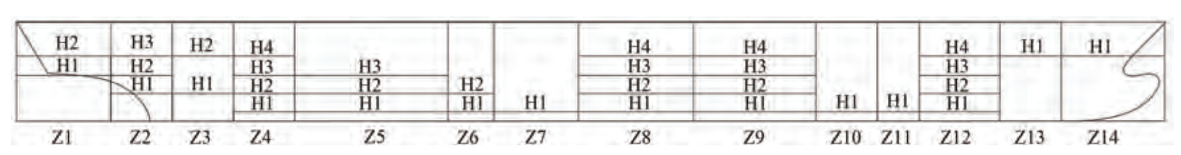 Figure 3 Effect drawing of vertical area division
After the above modeling is completed in Maxsurf software, the parameters are set, three calculation draft conditions are established, and the damaged area is set to complete the stability calculation of the damaged cabin. The results of the subdivision index are shown in Table 2. The three calculated draft conditions of the ship all meet the requirements of the convention, and the damage stability is good. Under light-load operation, the compartment index is 0.7195, and the damage stability is low.
Table 2 Calculation results of damaged stabilityName A R Pass/Fail As 0.980 2 0.606 87 Pass Ap 0.970 7 0.606 87 Pass Al 0.719 5 0.606 87 Pass A 0.924 3 0.674 3 Pass Statistical analysis of damage stability results: The damaged area with S < 1 was selected, the intermediate calculation process was deleted, and the longitudinal zone was merged. The data of the danger zone (the partial subdivision draught) is shown in Table 3. Statistics reveal six damaged zones in the deepest subdivision draught, nine in the partial subdivision draught, and 25 in the light-load operation subdivision draught.
Table 3 Data of danger zone for partial subdivision draftdanger zone Longitudinal midpoint position PRISK Part: Z3, 3; 61.3 0.000 884 Part: Z7, 3; 133.3 0.000 798 Part: Z2, 4; 54.9 0.003 076 Part: Z3, 4; 66.1 0.000 183 Part: Z4, 4; 81.3 0.000 767 Part: Z5, 4; 99.7 0.004 842 Part: Z6, 4; 128.5 0.000 627 Part: Z7, 4; 139.7 0.000 100 Part: Z8, 4; 152.9 0.000 063 3.1.2 Calculation of danger zone factor
A scatter diagram is established with the relative longitudinal position of the danger zone as the abscissa and the probability of damage as the ordinate (Figure 4) to quantify the relationship between the position of the ship's danger zone and the probability of damage. Curve fitting (Gaussian formula fitting) is performed on the scatter diagram. The fitting of danger zones under the deepest draught condition is shown in Figure 5.
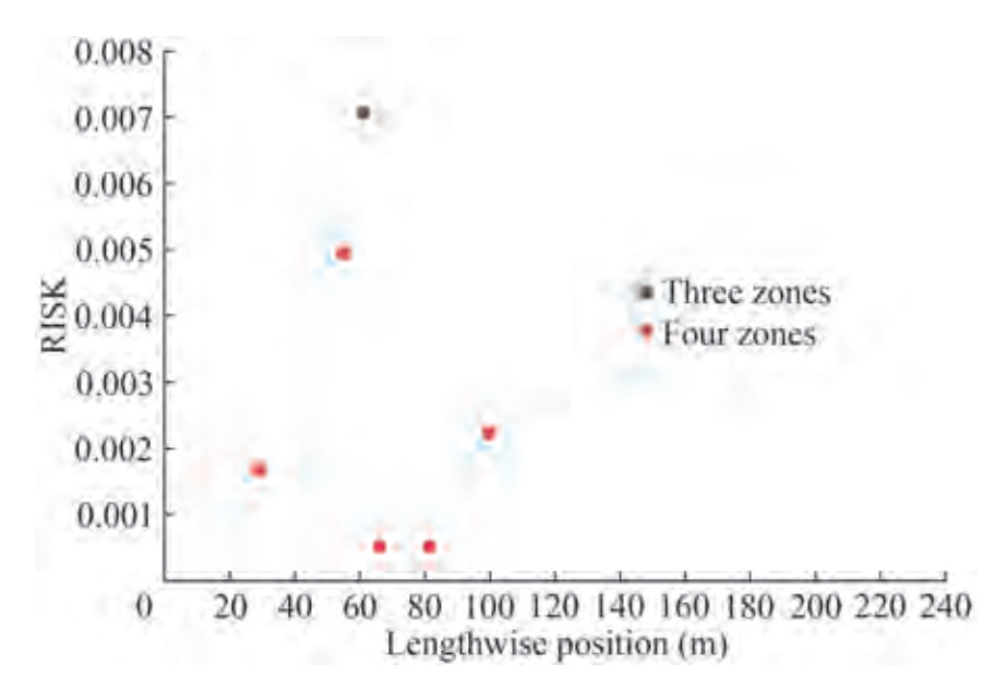 Figure 4 Distribution of the deepest subdivision draught danger zone
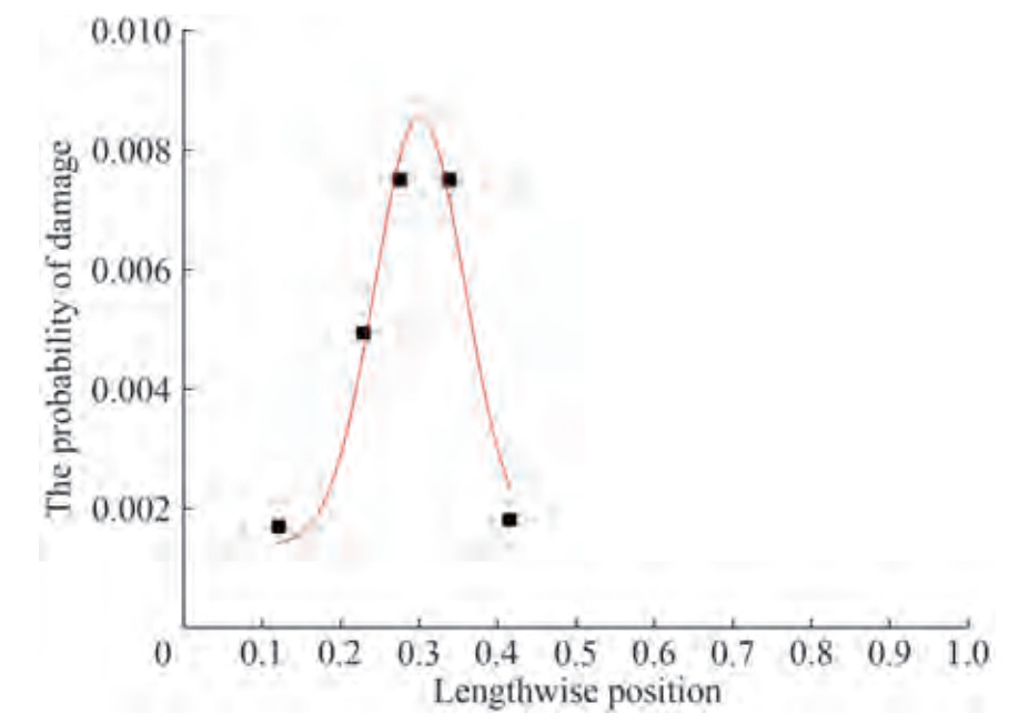 Figure 5 Data fitting diagram of deepest subdivision draught danger zones
The danger zone fitting of the deepest subdivision draft is as follows:
$$p = \\ \left\{ {\begin{array}{*{20}{l}} {0.00136 + \frac{{0.00103}}{{0.115 \times \sqrt {{\rm{ \mathsf{ π} }}/2} }}{e^{ - 2{{\left({\frac{{(x - 0.30)}}{{0.115}}} \right)}^2}}}(0.12 \leqslant x \leqslant 0.42)}\\ {0(0 \leqslant x \leqslant 0.12;0.42 \leqslant x \leqslant 1.0)} \end{array}} \right.$$ (8) where p is damage probability of the danger zone, x is center location of the danger zone.
The curve fitting data of danger zones of working conditions and the distribution of danger zones of partial compartment draft and curve fitting are shown in Figures 6 and 7, respectively.
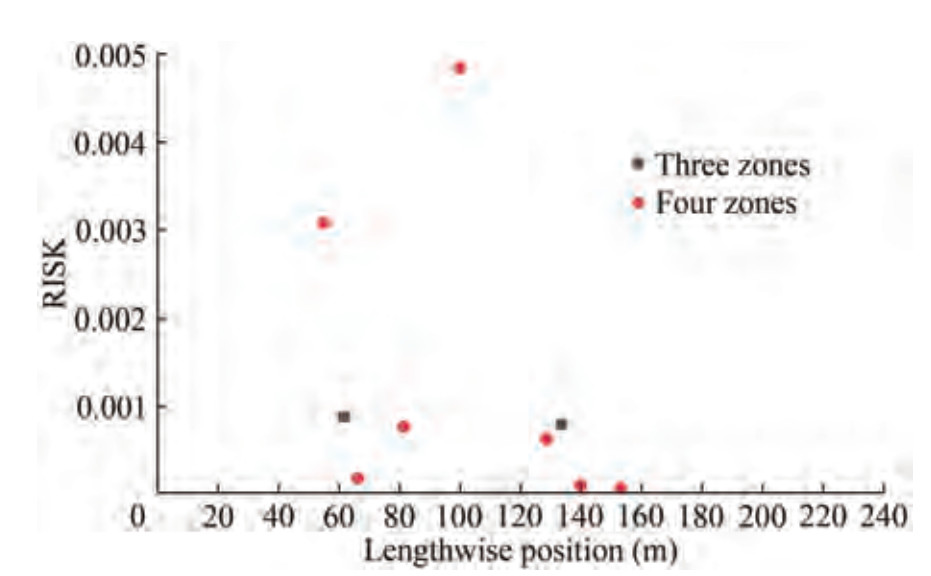 Figure 6 Distribution of partial subdivision draft danger zones
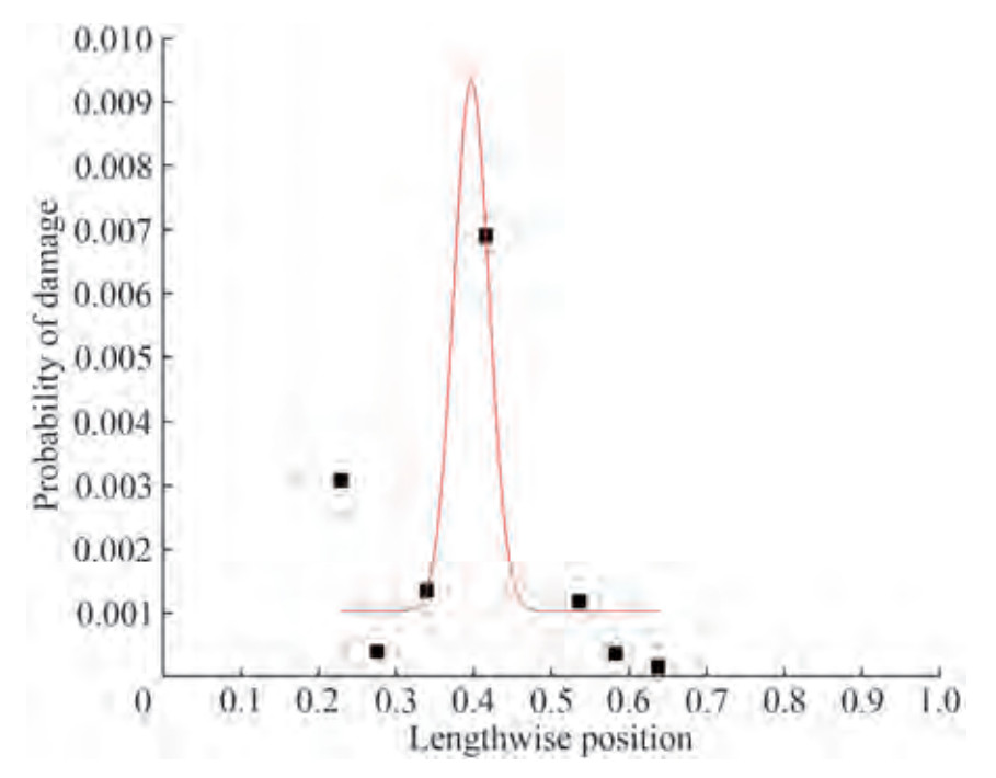 Figure 7 Data fitting diagram of partial subdivision draft danger zones
The danger zone fitting of the partial subdivision draught is as follows:
$$p =\\ \left\{ {\begin{array}{*{20}{l}} {0.00103 + \frac{{10.15}}{{859.2 \times \sqrt {{\rm{ \mathsf{ π} }}/2} }}{e^{ - 2{{\left({\frac{{x - 741}}{{8592}}} \right)}^2}}}(0.2 \leqslant x \leqslant 0.65)}\\ {0(0 \leqslant x \leqslant 0.2;0.65 \leqslant x \leqslant 1.0)} \end{array}} \right.$$ (9) Figure 8 shows the distribution of danger zones in light-load operation. The number of danger zones in light-load operation is 25, and damaged zones are found from a single zone to four zones. The most dangerous scene is the double-zone damage scene. Light-load operation subdivision draft danger zone fitting situation as shown in Figures 9–11.
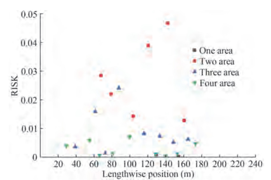 Figure 8 Distribution of danger zones in light-load operation subdivisions
 Figure 9 Fitting diagram of damage data in two zones
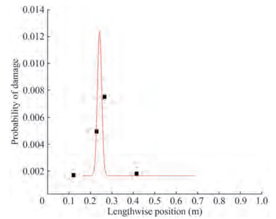 Figure 10 Fitting diagram of damage data in three zones
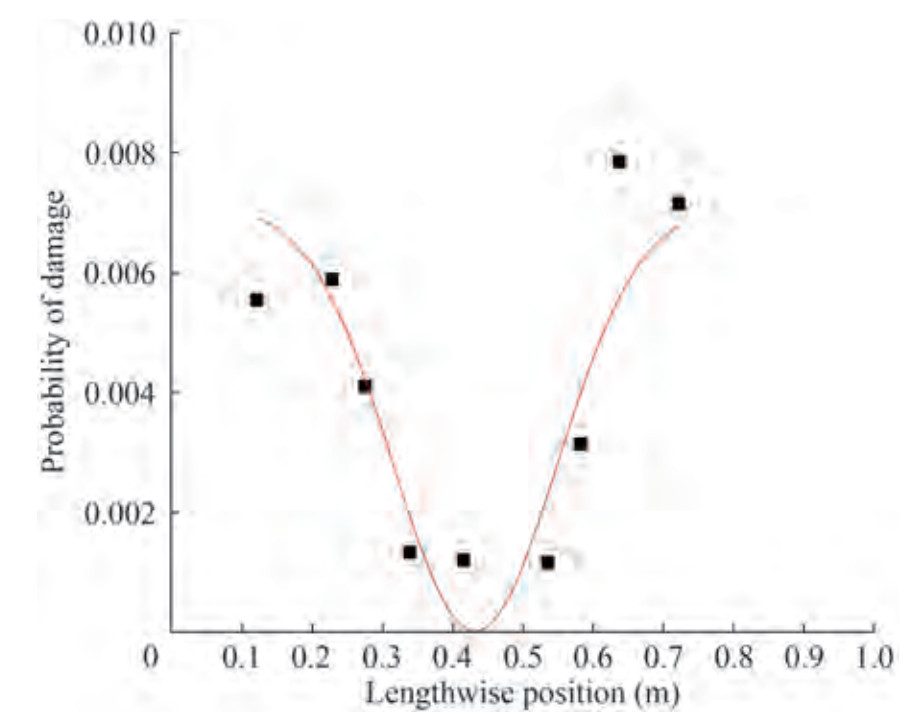 Figure 11 Fitting diagram of damage data in four zones
The damage fitting formulas of two, three, and four zones are respectively shown as Eqs. (10), (11), and (12).
$$p = \left\{ {\begin{array}{*{20}{l}} {0.0254 + \frac{{7940}}{{5518 \times \sqrt {{\rm{ \mathsf{ π} }}/2} }}{e^{ - 2{{\left({\frac{{(x - 538)}}{{5518}}} \right)}^2}}}}\\ {0(0 \leqslant x \leqslant 0.28;0.67 \leqslant x \leqslant 1.0)} \end{array}(0.28 \leqslant x \leqslant 0.67)} \right.$$ (10) $$p = \left\{ {\begin{array}{*{20}{l}} {0.00804 + \frac{{135.7}}{{439.2 \times \sqrt {{\rm{ \mathsf{ π} }}/2} }}{e^{ - 2{{\left({\frac{{(x - 78.69)}}{{439.2}}} \right)}^2}}}}\\ {0(0 \leqslant x \leqslant 0.16;0.68 \leqslant x \leqslant 1.0)} \end{array}(0.16 \leqslant x \leqslant 0.68)} \right.$$ (11) $$p = \left\{ {\begin{array}{*{20}{l}} {0.0071 + \frac{{ - 0.00209}}{{0.2344 \times \sqrt {{\rm{ \mathsf{ π} }}/2} }}{e^{ - 2{{\left({\frac{{(x - 0.4323)}}{{0.2344}}} \right)}^2}}}}\\ {0(0 \leqslant x \leqslant 0.12;0.72 \leqslant x \leqslant 1.0)} \end{array}\quad (0.12 \leqslant x \leqslant 0.72)} \right.$$ (12) The above analysis reveals that the Gaussian formula can effectively fit the relationship between the location of the danger zone of the ship and the damage probability.
$$p = {y_0} + \frac{A}{{\omega \times \sqrt {{\rm{ \mathsf{ π} }}/2} }}{e^{ - 2{{\left({\frac{{\left({x - {x_0}} \right)}}{\omega }} \right)}^2}}}$$ (13) where p is damage probability of the danger zone, x is center location of the danger zone.
Each coefficient is related to the general arrangement of the ship, and the parameters corresponding to different ship types and water inflow conditions are different. Each parameter can be determined by analyzing the damaged stability of the ship.
3.2 Calculation method of capsizing time factor
3.2.1 Calculation method of capsizing time based on monte carlo
The above analysis shows that the determination of capsizing time is the key to risk assessment. The time-domain simulation of water inflow can determine the capsizing time. Many random factors are found in the water inflow, and a large number of nearly ten thousand water inflow scenarios are the two significant problems of time-domain simulation. The Monte Carlo method is used in this paper to handle random factors and reasonably reduce the number of simulations.
Solving capsizing time by Monte Carlo simulation comprises two main parts: Monte Carlo sampling and numerical simulation. Monte Carlo sampling is used to determine the inflow case. First, analyzing and decomposing the influencing factors of the inflow case is necessary. The main influencing factors are loading conditions, damage area, and breach information (including the breach's shape, location, and size). The Monte Carlo sampling process is then identified as follows after determining the main influencing factors.
1) The random number "a" generated by the computer is used to determine the inflow condition: 0 ≤ a < 0.4 is the deepest subdivision draft; 0.4 ≤ a < 0.8 for partial subdivision draft; 0.8 ≤ a < 1.0 for light-load subdivision draft.
2) After the water inflow condition is identified, a random number "b" is generated to determine the damaged area. Most of the damages are minor accidents, which will not cause the ship to capsize but will occupy computing resources. This paper uses the risk index, Prisk, of a dangerous area to determine the damaged area and reduce the simulated sample.
$$\sum\limits_1^{j - 1} {{P_i}} \times \left({1 - {S_i}} \right) < b \leqslant \sum\limits_1^j {{P_i}} \times \left({1 - {S_i}} \right)\quad j = 1, \cdots, J$$ (14) where J is represents all danger zones.
If "b" satisfies the above conditions, then the damaged area is i; otherwise, the area is as follows:
$$b > \sum\limits_i^J {{P_i}} \times \left({1 - {S_i}} \right)$$ (15) Thus, the stability of the ship is sufficient after damage, and no risk is observed after water inflow.
3) After identifying the damaged area, the random number "c" is generated to determine the shape of the fracture. The shape and frequency of breaches have specific rules to follow. Based on the collision accident report published by the General Administration of Maritime Affairs of China, this paper found 92 effective damage cases, and the frequency of each shape breach is shown in Table 4.
Table 4 Statistical table of break shapeShape Number Square 8 Circular 14 Vertical strip 6 Longitudinal strip 48 Rotated square 16 Total 92 4) The random number "d " is used to determine the position of the break. The break can theoretically appear at any position of the damaged outer plate. The break position adopts uniform distribution considering this randomness.
All the above information is integrated to obtain an influx case. The random simulation of the following inflow condition is then conducted, and all the issues to be simulated can be obtained by counting the sampling results. The time-domain simulation of the model case can obtain the capsizing time.
The above Monte Carlo sampling program was used to determine the simulated ship inflow cases, 200 samplings were conducted, and the sampling results were statistically analyzed. A total of 11 cases to be simulated (cases with dumping risk after inflow) were obtained, as shown in Table 5.
Table 5 Break information for simulated casesDamaged zones Load case Break shape Break shape Break shape Relative position Relative position Relative position Z5, 6 Light Longitudinal Circular strip 0.53 0.39 0.9 0.04 Z8, 9 Light Longitudinal Longitudinal strip strip 0.57 0.71 0.89 0.02 Z5, 6, 7, 8 Part Circular Longitudinal Longitudinal 0.89 0.22 strip strip 0.17 0.12 0.22 0.15 Z3, 4, 5 Deep Longitudinal Longitudinal Longitudinal strip strip strip 0.47 0.03 0.63 0.07 0.41 0.28 Z5, 6, 7 Light Circular Rotated Rotated square 0.41 0.04 square 0.24 0.25 0.4 0.28 Z8 Light Circular 0.03 0.64 Z7, 8, 9 Part Longitudinal Longitudinal Rotated square strip strip 0.25 0.36 0.74 0.36 0.53 0.73 Z8, 9 Light Circular Longitudinal 0.06 0.31 strip 0.53 0.88 Z8, 9 Light Rotated square Longitudinal 0.57 0.71 strip 0.89 0.02 Z5, 6 Light Longitudinal Longitudinal strip strip 0.03 0.85 0.32 0.2 Z4, 5 Light Longitudinal Longitudinal strip strip 0.41 0.8 0.41 0.8 Notably, this paper assumes a breach in each zone, and the breach area is 9 m2. The relative position represents the relative coordinates of the fracture in the current length and height direction of the damaged zone.
The use of CFD technology to study ship inflow has currently become mainstream. Thus, time-domain simulation must follow the conservation of mass and momentum. In this section, the VOF method captures the water–air interface, and dynamic grid technology is used to predict the floating state of the ship. Fluent software is used to indicate the floating state of the ship after entering the water. This software divides the solution domain into a finite number of adjacent control bodies and applies the conservation equation to each control body.
$$\int_V {\frac{\partial }{{\partial t}}} (\rho \phi){\rm{d}}v + \int_V {{\mathop{\rm div}\nolimits} } (\rho v\phi){\rm{d}}v = \int_V {{\mathop{\rm div}\nolimits} } (\Gamma {\mathop{\rm grad}\nolimits} \phi){\rm{d}}v + \int_V S {\rm{d}}v$$ (16) where ϕ is niversal variable, V is control volume, Γ is generalized diffusion coefficient, S is generalized the source term.
First, a simple box cabin verifies the accuracy of CFD time-domain simulation. The cabin size is 8 m × 4 m × 4 m, and the internal watertight plate is divided into four cabins. The breach is located on the starboard side, as shown in Figure 12. In this case, the water inflow time was 65 s, and the water inflow was 2 937 kg. The motion curve is shown in Figure 13.
 Figure 12 Section diagram of cabin structure
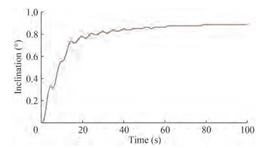 Figure 13 Cabin trim curve
The equal large box cabin is then established using the ship performance analysis software Maxsurf. Under this damaged condition, the stern inclination of the cabin is 0.065 m, and the inclination angle is 0.93°. The difference between the two results is 6.55%, and the error is acceptable.
Take the water inflow in Z8 and Z9 areas as an example. Z8 and Z9 areas are water inflow areas, and the position of the longitudinal watertight plate is 117 m-141 m-167 m. The watertight partition board is established, and two breaches are observed. The first breach is a circular breach, r = 1.7 m, and the relative position of the center is (0.06, 0.31). Therefore, the coordinates of the breach center are (−0.1, −6.1, 16). The second breach is a longitudinal strip with a dimension of 4.2 × 2.1 (m). The center coordinates are (34.7, −3.8, 16). The inflow model is shown in Figure 14.
 Figure 14 Z8, 9 inflow model
The computing domain is established, the grid is divided, and relevant settings are set up for simulation. The sorting result shows that the water inflow time of the ship is 667 s, and the final flooding quantity is 8 972 656 kg. In this model, the water inflow is large, and the bow inclination ship is enormous. Finally, the bow inclination angle of the ship reaches 2.8° at 667 s. The main deck of the ship has already waded and begun to abandon the ship. The capsizing time of this case is 667 s. The cases obtained by Monte Carlo sampling were modeled and simulated in the time-domain, and the results are shown in Table 6.
Table 6 Statistical table of water inflow time-domain simulation resultsNumber Load case Final inflow (kg) Capsize or not Capsize/inlet time (s) 1 Light 3 273 782 No 420 2 Light 7 540 062 No 496 3 Light 9 699 273 Yes 688 4 Light 8 972 656 Yes 667 5 Part 10 649 240 Yes 593 6 Part 12 403 238 Yes 578 7 Light 9 535 050 Yes 602 8 Light 5 010 542 No 580 9 Light 9 540 953 No 458 10 Light 6 126 682 Yes 711 11 Deep 15 131 486 Yes 687 3.2.2 Calculation of capsizing time factor
The break is the main factor affecting the inlet velocity, and the inlet velocity directly affects the inlet process. Studying the relationship between the break area, shape, location, and inlet velocity is essential. The decomposition of break characteristics is analyzed in accordance with Section 3.2.1. The box cabin is taken as the research object (6 m× 4 m× 5 m) for analysis to save computational resources.
3.2.2.1 Area
Taking the square breach as an example, the areas of 0.25, 1, and 2.25 m2 are selected, and the parameters are the same. The inflow cases with different breach areas were simulated. The average inflow speed in different periods was calculated to obtain the relationship between the breach area and the inflow speed quantitatively, as shown in Figure 15.
 Figure 15 Variation of inflow velocity
Figure 15 shows a positive correlation between the break area and the inflow velocity per unit area, which can be expressed as follows:
$${{V = k S}}$$ (17) where V is inflow velocity per unit area, k is proportionality factor, S is break area.
3.2.2.2 Center height
The height of the center position is 0.5, 0, −0.5, −1, and −1.5 m (draft is 1 m). The inflow velocity in different periods is calculated as shown in Figure 16.
 Figure 16 Variation of inflow velocity
Figure 16 reveals that the breaking height has minimal effect on the average inlet velocity of large openings.
3.2.2.3 Longitudinal position
The broken mouth is square and the area is 1 m2. The longitudinal position of the broken mouth center is −2, 0, and 2 m. The inflow velocity changes with the longitudinal position as shown in Figure 17.
 Figure 17 Variation of inflow velocity
The inlet velocity in the middle of the breach is the largest, and the inlet velocity in the head and tail are symmetrically distributed. The inlet velocity per unit area at different positions is linearly related to the reference velocity based on the velocity position of the center point.
$${{V = k|x| + b}}$$ (18) where V is inflow velocity per unit area, x is relative position of the break center point, b is inlet velocity at the longitudinal central break.
3.2.2.4 Shape
The break shape reference is presented in Table 4, the break area is 1 m2, and the break center position is (0, 0, 3). The inflow velocity is shown in Table 7. The table reveals that the inlet velocity from high to low is as follows: vertical strip break, oblique square, square, circular, and transverse strip break.
Table 7 Inlet velocity of different shapes of breaches(m/s) Break shape Shape factors 3 s 5 s 7 s 9 s Circular 0.56 1.7 1.9 1.9 1.9 Square 1 1.9 1.9 1.9 1.9 Vertical strip 2 3.1 3.2 3.2 3.2 Rotated square 1.41 1.9 2.1 2.1 2.1 Longitudinal strip 0.5 1.3 1.3 1.3 1.3 In the same area, a large vertical proportion of the break induces a large inflow velocity. The breach shape factor γ is used to quantify the impact of the shape factor on the inflow velocity. The solution formula of shape factor can be defined:
$$\gamma = \frac{H}{{\sqrt S }}$$ (19) where γ is shape factor, H is longest vertical distance of the breach, S is break area.
The scatter plot reveals that this relationship has minimal adaptability at the round break, and the scatter fitting after excluding the round break is shown in Figure 18.
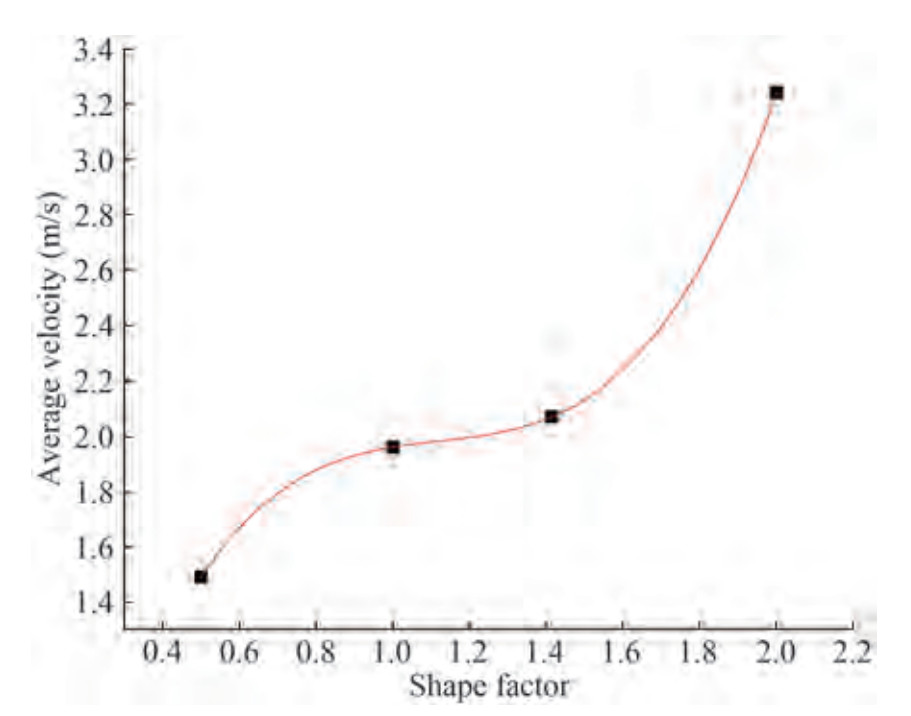 Figure 18 Fitting diagram of break shape factor
The fitted functional relationship is as follows:
$$V = a + {k_1}\gamma - {k_2}{\gamma ^2} + {k_3}{\gamma ^3}$$ (20) The influence of the above break information on the inlet velocity can be sorted out as the correction value to correct the reference velocity. The reference correction value selects the square break located in the longitudinal middle of the unit area. The function relation between inlet velocity, inlet time, and break information can be obtained by Eqs. (17), (18), (19), and (20).
$$\begin{array}{c} V = {\beta _1}S\left({{\beta _2}|x| + {V_0}} \right) \times \\ \frac{{a + {k_1}\frac{H}{{\sqrt S }} - {k_2}{{\left({\frac{H}{{\sqrt S }}} \right)}^2} + {k_3}{{\left({\frac{H}{{\sqrt S }}} \right)}^3}}}{{a + {k_1} - {k_2} + {k_3}}} \end{array}$$ (21) $$\begin{array}{l} t = \\ \frac{Q}{{{\beta _1}{S^2}\left({{\beta _2}|x| + {V_0}} \right) \times \frac{{a + {k_1}\frac{H}{{\sqrt S }} - {k_2}{{\left({\frac{H}{{\sqrt S }}} \right)}^2} + {k_3}{{\left({\frac{H}{{\sqrt S }}} \right)}^3}}}{{a + {k_1} - {k_2} + {k_3}}}}} \end{array}$$ (22) where V is intake velocity per unit area; t is inlet time; Q is flooding quantity; S is break area; β1 is the correction coefficient of the broken area is the same as k in Eq. (23); β2 is the correction coefficient of the longitudinal position of the breach is the same as that in Eq. (24); H is longest vertical distance of the breach; a, k1, k2, k3 are the correction parameters of notch shape to velocity.
Eqs. (21) and (22) construct the functional relationship between the area, position, and shape of the break and the inlet velocity and time. The area of the break has the largest impact on the inlet velocity, followed by the shape of the break (the longest vertical distance). The above formula can essentially help understand the influencing factors of inflow time.
3.3 Calculation method of the evacuation time factor
3.3.1 Evacuation capability in ship water inflow
Evacuation capacity is an important index to measure whether people can evacuate safely after accidents, such as flooding, and is also an essential parameter in quantitative risk assessment. The evacuation of personnel can be summarized as transferring personnel from the ship to the lifeboat. After the ship enters the water, the ship will produce a roll or pitch motion under the action of waves and internal moisture, which will affect the evacuation process of personnel. Brumley (2000) sorted the influence of ship inclination on personnel speed into an inclination coefficient to correct personnel speed.
$$V = {V_0} \times {k_1}$$ (23) where V is speed, individual actual speed; V0 is initial speed, the speed of individuals moving on flat ground; k1 is inclination coefficient, which is the ratio of the speed of an individual at a specific inclination angle to that of an individual on flat ground.
The personnel evacuation software Exodus can simulate individual behaviors and hull details. Exodus is based on the principle of cellular automata. This software can simulate the process of multiple people evacuating in an enormous ship geometry by establishing the walking ground field of personnel based on the exit location and setting the behavior models of personnel social force, group influence, personnel attribute classification influence, and hull motion; it can also couple fire data, toxic gas, and inclination angle (Owen et al. 1996; Veeraswamy et al. 2018). The model considers the effects of people, people and fire, and people and structure.
First, the personnel evacuation simulation model is established, as shown in Figure 19. The initial position of personnel is then set, and the emergency condition at night is selected, under which all passengers are in the living quarters: one-third of the crew is located in the working area of the ship, and two-thirds are located in the cabin of the crew. The personnel properties are shown in Table 8.
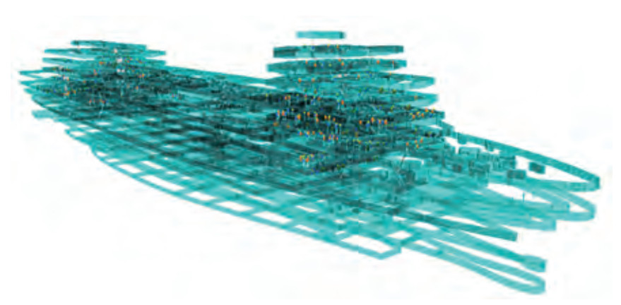 Figure 19 3D evacuation sceneTable 8 Personnel attributes
Attribute characteristics Average Min Max Age 38.85 20.00 59.00 Agility degree 5.04 3.01 7.00 Motivation 7.61 1.07 14.91 Fast walking (m/s) 1.14 0.80 1.50 Walk (m/s) 1.02 0.72 1.35 creep (m/s) 0.23 0.16 0.30 Jump (m/s) 0.91 0.64 1.20 Mobility 1.00 1.00 1.00 Weight (kg) 61.80 49.53 74.97 The ship motion data are coupled with the personnel evacuation as the deck inclination data after the ship enters the water. The evacuation of the ship in static and inclined states is simulated. The statistical evacuation results are shown in Figure 20.
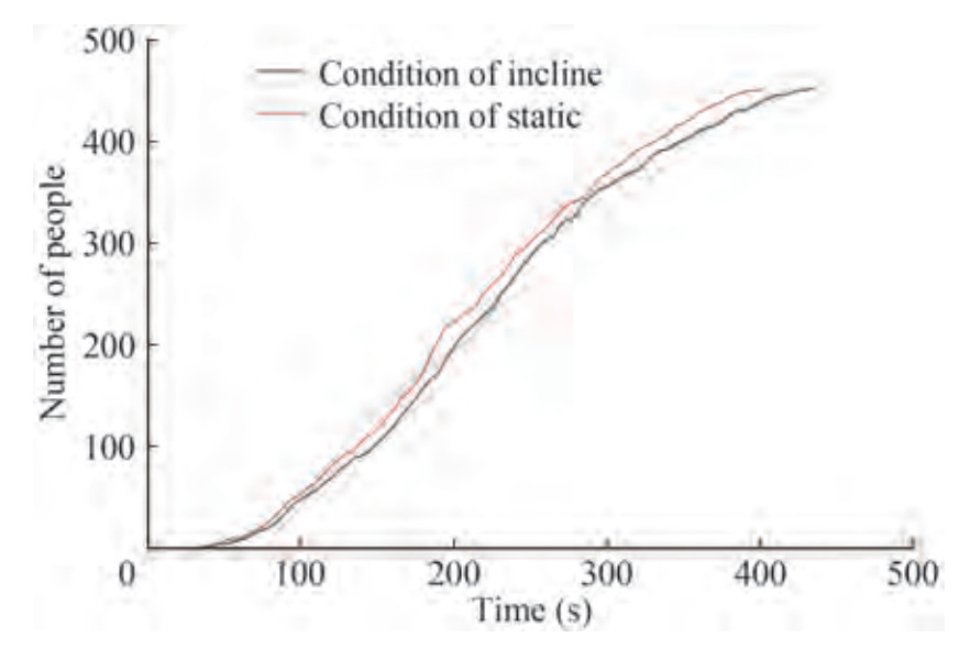 Figure 20 Comparison of evacuation curves
All deck evacuation times are shown in Table 9.
Table 9 Evacuation time for each deckDeck name Evacuation time-static (s) Evacuation time-incline (s) Delay ratio (%) Bottom cabin 33 35 6.1 2 Deck 84 90 7.1 1 Deck 260 305 17.3 01 Deck 402 433 7.7 02 Deck 229 230 0.4 03 Deck 103 110 6.8 04 Deck 61 63 3.3 05 Deck 54 55 1.9 06 Deck 37 38 2.7 The hull inclination affects the evacuation time of all decks, and the delay effect on deck 1 is the most evident, with a delay of 17.3%. The final and longitudinal rolls of the ship are 6.5° and 1.8°, respectively. The change in the floating state, the influence on the personnel speed, and the impact on the evacuation results are all small. The coupling of the motion curve and the evacuation can help obtain the evacuation situation in the ship water inflow.
3.3.2 Calculation of evacuation time factor
The influence of the water environment on the evacuation time is converted into the relationship between the ship inclination angle and the evacuation time. The influence of different inclination types and angles on the evacuation time is solved on the basis of the Exodus platform. Taking the evacuation time of the ship's floating state as the benchmark, the evacuation delay effect of different inclination angles is calculated. The results are shown in Table 10. The relationship between inclination angle and delay time is shown in Figures 21 and 22. These figures reveal that the delay effect is linear with the inclination angle.
$$\delta = k\theta $$ (24) Table 10 Influence of heeling on evacuation timeInclination angle (heel) (°) Evacuation time (s) Delay ratio (%) −20 500 24.4 −15 483 20.1 −10 453 12.7 −5 427 6.2 0 402 0.0 5 414 2.9 10 428 6.5 15 442 9.9 20 455 13.%  Figure 21 Scatter diagram of heeling angle and delayed evacuation effect
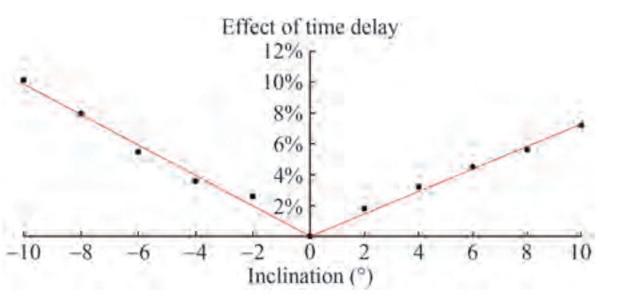 Figure 22 Scatter diagram of trim angle and delayed evacuation effect
where δ is delay effect (based on the evacuation of ship floating state), k is scale factor, θ is inclination degree.
The value of the proportional coefficient can be obtained by fitting Figures 21 and 22 (the ship's right inclination is positive): in the case of left inclination: δ = −0.001 3θ; in the case of right inclination: δ = 0.000 65θ; in the case of bow inclination: δ = −0.009 9θ; in the case of stern inclination: δ = 0.007 3θ.
The proportional coefficient reveals that inclination has minimal effect on evacuation; at the same inclination angle, the influence of the bow on evacuation is more evident than that of the tail, and the influence of the left on evacuation is more evident than that of the right. The proportional coefficient can quantify the impact of different types of inclination (stern, bow, right, and left inclinations) on delayed evacuation.
3.4 Total risk model
Overall, the danger zone, capsizing time, and evacuation factors can be integrated. Based on the background of ship inflow, the danger zone, capsizing time, and evacuation time factors can be reflected in the risk model of ship inflow. Combined with the risk model shown in Eq. (4), the risk can be finally classified into two main factors: the location of the damaged zone and the breached information.
$${p_i} = {y_0} + \frac{A}{{\omega \times \sqrt {{\rm{ \mathsf{ π} }}/2} }}{e^{ - 2{{\left({\frac{{\left({x - {x_0}} \right)}}{\omega }} \right)}^2}}}$$ (25) $$\begin{array}{l} {\varepsilon _{i, j}}\left({{t_{{\rm{cap }}}}} \right) = {\varepsilon _{i, j}}\\ \left({\frac{Q}{{{\beta _1}{S^2}\left({{\beta _2}|x| + {V_0}} \right) \times \frac{{a + {k_1}\frac{H}{{\sqrt S }} - {k_2}{{\left({\frac{H}{{\sqrt S }}} \right)}^2} + {k_3}{{\left({\frac{H}{{\sqrt S }}} \right)}^3}}}{{a + {k_1} - {k_2} + {k_3}}}}}} \right) \end{array}$$ (26) where p is damage probability of danger zones; x is center location of danger zones; εi, j (tcap) is number of deaths in i, j events; ω, x0 are considering the general arrangement of the ship, each parameter can be determined by analyzing the stability of the ship; V is inflow velocity per unit area; t is inlet time; S is break area; β1 is correction coefficient of the broken area; β2 is correction coefficient of the longitudinal position of the breach; H is longest vertical distance of the breach; a, k1, k2, k3 are correction coefficients of break shape to velocity.
The above formula indicates that the longitudinal position of the damaged zone and the breach area significantly impacts the risk. However, the broken area cannot be determined before the accident. Therefore, reducing the damage probability of the ship is the best way to control the aforementioned phenomenon. The damage probability of the danger zone of the ship is related to the general layout. Given this phenomenon, the local general layout can be adjusted to reduce the probability of ship damage and the risk of the ship.
4 Cabin division optimization based on risk loss
4.1 Selection of zone to be optimized based on risk loss
Risk reduction has always been the goal of designers. After the preliminary design of the ship is completed, redesigning the general layout of the ship to reduce the risk of the ship is not feasible. At this time, the ship design has met the performance of other ships. Local adjustment is the first choice to reduce the risk without changing the overall performance of the ship.
Seven capsizing scenarios are obtained in Section 3.2.1. The casualty problem is an indicator to measure the risk. The time-domain simulation of ship inflow and evacuation analysis show that when the ship capsizing occurs, if some people fail to complete the evacuation before the capsizing time, then a risk of casualties is possible. The number of deaths can be determined by taking the dumping time of the dumping scene as the input of the evacuation curve. Taking Condition 1 in Table 11 as an example, the evacuation curve is shown in Figure 23. The reaction time was 5 min, and people began to escape in 335 s. A total of 414 people completed their evacuation in 667 s of dumping. The 38 remaining people were left on the ship, and the number of deaths in this scene was 38. The number of deaths in seven capsizing scenarios is counted as shown in Table 11.
Table 11 Statistics of casualties in capsizing scenesLoad case damage zone Damage probability Number of deaths Risk loss 1 Z8, 9-light 0.046 724 23 2.78E-03 2 Z8, 9-light 0.046 724 38 4.60E-03 3 Z7, 8, 9-part 0.007 282 95 1.79E-03 4 Z5, 6, 7, 8-Part 0.006 902 113 2.01E-03 5 Z5, 6, 7-light 0.024 066 81 5.03E-03 6 Z3, 4, 5-deep 0.007 051 5 9.10E-05 7 Z4, 5, 6, 7-light 0.035 138 0 2.78E-03 Note: Risk loss is obtained by multiplying the occurrence probability P of the inflow scenario with the number of deaths N. 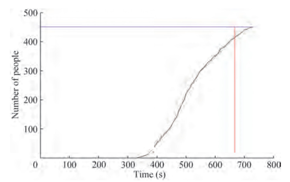 Figure 23 Personnel evacuation curve in capsizing scenario
Table 11 shows that the risk value of working condition 2 and the risk loss of working condition 5 is the largest. Working conditions 1 and 2 are damaged in Z8 and Z9 zones, and the risk of damage in Z8 and Z9 zones is the largest. Hence, Z8 and 9 are the zones to be optimized.
4.2 Optimization performance calculation
Zones Z8 and 9 are the zones to be optimized. Eqs. (25) and (26) reveal that the longitudinal position of the damaged area and the area of the breach has the most significant impact on the risk, and the area of the breach cannot be determined before the accident. Adjusting the longitudinal position of the watertight plates in areas Z8 and 9 is the best method to be controlled. The longitudinal position of the two regions is 117.3 m-141.3 m-166.9 m. The position of the watertight compartment plate in the middle of Z8, 9 is adjusted to form an optimization scheme to maintain the position information of the compartment.
First, determining the moving direction of the watertight plate is necessary. The length of the entire ship should also be maintained. Scheme 1: the subdivision watertight plate position in the middle of Z8 and Z9 is moved to the stern 1 m; Scheme 2: the subdivision watertight plate position in the middle of Z8 and Z9 is moved to the bow 1 m. Maxsurf software was used to remodel the two optimization schemes, and the damage stability was evaluated. The damage stability evaluation results and the damage probability of Z8 and Z9 regions were counted in accordance with the damage stability evaluation results, as shown in Table 12.
Table 12 Comparison of damaged stability resultsName Original model Scheme 1 Scheme 2 AS 0.964 665 0.981 189 0.960 379 AP 0.967 13 0.978 573 0.960 520 AL 0.715 86 0.769 919 0.712 800 A 0.915 89 0.937 889 0.910 924 p 0.046 724 0.046 442 0.046 829 Table 12 reveals that scheme 1 has an increase in the subdivision index and a decrease in the probability of damage compared with the original model, and scheme 2 has a reduction in the subdivision index and an increase in the probability of damage compared with the original model. Therefore, for this ship, moving the position of the subdivision watertight plate in the middle of Z8 and Z9 to the stern can reduce the probability of damage and improve the subdivision index. Supplementary optimization schemes: a) scheme 3: the length of the entire ship is maintained, and the position of the subdivision watertight plate in the middle of Z8 and Z9 is moved to the stern by 0.5 m; b) scheme 4: the position of the subdivision watertight plate in the middle of Z8 and Z9 is moved to the stern by 1.5 m. The above scheme only adjusts the local area of the ship; therefore, this scheme mainly considers the changes in the initial stability and floating state of the ship. Maxsurf software is used in the calculation under the complete load condition. The statistical differences between the initial floating state and the initial metacentric height are shown in Table 13.
Table 13 Calculation results of initial floating state and high initial stability of each schemeScheme Trim (m) GM (m) Original model 0.095 2.098 Scheme 1 0.067 2.104 Scheme 2 0.123 2.094 Scheme 3 0.081 2.100 Scheme 4 0.054 2.099 The reassessment of damage stability, the results of the damage stability assessment, and the damage probability of Z8 and Z9 zones are shown in Table 14.
Table 14 Comparison of damage stability results and damage probability of each schemeName Original model Scheme 1 Scheme 3 Scheme 4 AS 0.964 665 0.981 189 0.965 275 0.965 189 AP 0.967 13 0.978 573 0.967 587 0.968 578 AL 0.715 86 0.769 919 0.715 923 0.715 921 A 0.915 89 0.937 889 0.916 330 0.916 691 p 0.046 724 0.046 442 0.046 707 0.046 593 Table 14 reveals that schemes 3 and 4 have increased subdivision index and decreased damage probability compared with the original scheme, but the impact is negligible. Compared with other schemes, scheme 1 has a significant effect on the increase in subdivision index and the decrease in damage probability of the original model. Therefore, scheme 1 is finally determined as the final optimization scheme.
The risk assessment of scheme 1 is conducted, and the breach and marine information are consistent with the original model. The risk assessment results are shown in Table 15.
Table 15 Comparison table of inflow results of the optimization modelModel Original model Optimized model Flooding quantity (kg) 8 972 656 76 174 79 Inflow time Tcap (s) 667 727 Evacuation time Tevac (s) 729 712 Number of deaths 38 0 The optimized model: the water inflow process slows down, the final inflow quantity decreases, the water inflow time increases, the water inflow process is delayed, the water inflow time is 727 s, and the water inflow process finally does not overturn. Simultaneously, the personnel evacuation time is reduced to 712 s. In this scenario, all personnel are successfully evacuated with no casualties. The FN curve is illustrated as shown in Figure 24. The curve reveals that the social risk of the optimized ship is reduced.
 Figure 24 FN curve comparison
5 Conclusions
This paper proposes a DCEFM to quantify the risk of ship inflow. The probability of ship damage stability is evaluated on the basis of SOLAS 2020. Based on the concept of a danger zone, the curve fitting of danger zone data is performed, and the functional relationship between the probability of danger zone damage and the longitudinal position is obtained. The time-domain simulation method of damaged water in real ships is constructed on the basis of CFD. The influence of breach area, height, longitudinal position, and shape on the water velocity is obtained through the water simulation of various types of breaches. The empirical formula is fitted to simplify the influence of the water process on tilting time. Based on the inclined evacuation experiment and the ship evacuation mechanism, the influence of the water inflow on the evacuation is classified as the correction of the deck inclination to the personnel speed. The influence of various factors on the risk is analyzed in accordance with the DCEFM total risk model. The results show that the longitudinal position of the damaged and breached areas has the greatest impact on the risk. Risk loss value is used to evaluate the risk of capsizing scenarios. A simple local watertight plate position adjustment is performed in the high-risk value area to form an optimization scheme. The optimization performance calculation results show that the risk of ship water inflow can be reduced.
This paper selects the zone to be optimized on the basis of quantitative risk loss. Only a few optimization schemes are proposed due to the limited space of this paper and the emphasis on the combination of methods. The subsequent research intends to increase the optimization scheme, study the contribution of different optimization schemes to improve safety, and obtain the optimal optimization design scheme.
-
Figure 1 Calculation process of damage stability
Figure 2 Division effect chart of ship cabin
Figure 3 Effect drawing of vertical area division
Figure 4 Distribution of the deepest subdivision draught danger zone
Figure 5 Data fitting diagram of deepest subdivision draught danger zones
Figure 6 Distribution of partial subdivision draft danger zones
Figure 7 Data fitting diagram of partial subdivision draft danger zones
Figure 8 Distribution of danger zones in light-load operation subdivisions
Figure 9 Fitting diagram of damage data in two zones
Figure 10 Fitting diagram of damage data in three zones
Figure 11 Fitting diagram of damage data in four zones
Figure 12 Section diagram of cabin structure
Figure 13 Cabin trim curve
Figure 14 Z8, 9 inflow model
Figure 15 Variation of inflow velocity
Figure 16 Variation of inflow velocity
Figure 17 Variation of inflow velocity
Figure 18 Fitting diagram of break shape factor
Figure 19 3D evacuation scene
Figure 20 Comparison of evacuation curves
Figure 21 Scatter diagram of heeling angle and delayed evacuation effect
Figure 22 Scatter diagram of trim angle and delayed evacuation effect
Figure 23 Personnel evacuation curve in capsizing scenario
Figure 24 FN curve comparison
Table 1 Main scale parameters of ship
(m) Length 240 Beam 32 Height 17.5 Design draft 10.8 Table 2 Calculation results of damaged stability
Name A R Pass/Fail As 0.980 2 0.606 87 Pass Ap 0.970 7 0.606 87 Pass Al 0.719 5 0.606 87 Pass A 0.924 3 0.674 3 Pass Table 3 Data of danger zone for partial subdivision draft
danger zone Longitudinal midpoint position PRISK Part: Z3, 3; 61.3 0.000 884 Part: Z7, 3; 133.3 0.000 798 Part: Z2, 4; 54.9 0.003 076 Part: Z3, 4; 66.1 0.000 183 Part: Z4, 4; 81.3 0.000 767 Part: Z5, 4; 99.7 0.004 842 Part: Z6, 4; 128.5 0.000 627 Part: Z7, 4; 139.7 0.000 100 Part: Z8, 4; 152.9 0.000 063 Table 4 Statistical table of break shape
Shape Number Square 8 Circular 14 Vertical strip 6 Longitudinal strip 48 Rotated square 16 Total 92 Table 5 Break information for simulated cases
Damaged zones Load case Break shape Break shape Break shape Relative position Relative position Relative position Z5, 6 Light Longitudinal Circular strip 0.53 0.39 0.9 0.04 Z8, 9 Light Longitudinal Longitudinal strip strip 0.57 0.71 0.89 0.02 Z5, 6, 7, 8 Part Circular Longitudinal Longitudinal 0.89 0.22 strip strip 0.17 0.12 0.22 0.15 Z3, 4, 5 Deep Longitudinal Longitudinal Longitudinal strip strip strip 0.47 0.03 0.63 0.07 0.41 0.28 Z5, 6, 7 Light Circular Rotated Rotated square 0.41 0.04 square 0.24 0.25 0.4 0.28 Z8 Light Circular 0.03 0.64 Z7, 8, 9 Part Longitudinal Longitudinal Rotated square strip strip 0.25 0.36 0.74 0.36 0.53 0.73 Z8, 9 Light Circular Longitudinal 0.06 0.31 strip 0.53 0.88 Z8, 9 Light Rotated square Longitudinal 0.57 0.71 strip 0.89 0.02 Z5, 6 Light Longitudinal Longitudinal strip strip 0.03 0.85 0.32 0.2 Z4, 5 Light Longitudinal Longitudinal strip strip 0.41 0.8 0.41 0.8 Table 6 Statistical table of water inflow time-domain simulation results
Number Load case Final inflow (kg) Capsize or not Capsize/inlet time (s) 1 Light 3 273 782 No 420 2 Light 7 540 062 No 496 3 Light 9 699 273 Yes 688 4 Light 8 972 656 Yes 667 5 Part 10 649 240 Yes 593 6 Part 12 403 238 Yes 578 7 Light 9 535 050 Yes 602 8 Light 5 010 542 No 580 9 Light 9 540 953 No 458 10 Light 6 126 682 Yes 711 11 Deep 15 131 486 Yes 687 Table 7 Inlet velocity of different shapes of breaches
(m/s) Break shape Shape factors 3 s 5 s 7 s 9 s Circular 0.56 1.7 1.9 1.9 1.9 Square 1 1.9 1.9 1.9 1.9 Vertical strip 2 3.1 3.2 3.2 3.2 Rotated square 1.41 1.9 2.1 2.1 2.1 Longitudinal strip 0.5 1.3 1.3 1.3 1.3 Table 8 Personnel attributes
Attribute characteristics Average Min Max Age 38.85 20.00 59.00 Agility degree 5.04 3.01 7.00 Motivation 7.61 1.07 14.91 Fast walking (m/s) 1.14 0.80 1.50 Walk (m/s) 1.02 0.72 1.35 creep (m/s) 0.23 0.16 0.30 Jump (m/s) 0.91 0.64 1.20 Mobility 1.00 1.00 1.00 Weight (kg) 61.80 49.53 74.97 Table 9 Evacuation time for each deck
Deck name Evacuation time-static (s) Evacuation time-incline (s) Delay ratio (%) Bottom cabin 33 35 6.1 2 Deck 84 90 7.1 1 Deck 260 305 17.3 01 Deck 402 433 7.7 02 Deck 229 230 0.4 03 Deck 103 110 6.8 04 Deck 61 63 3.3 05 Deck 54 55 1.9 06 Deck 37 38 2.7 Table 10 Influence of heeling on evacuation time
Inclination angle (heel) (°) Evacuation time (s) Delay ratio (%) −20 500 24.4 −15 483 20.1 −10 453 12.7 −5 427 6.2 0 402 0.0 5 414 2.9 10 428 6.5 15 442 9.9 20 455 13.% Table 11 Statistics of casualties in capsizing scenes
Load case damage zone Damage probability Number of deaths Risk loss 1 Z8, 9-light 0.046 724 23 2.78E-03 2 Z8, 9-light 0.046 724 38 4.60E-03 3 Z7, 8, 9-part 0.007 282 95 1.79E-03 4 Z5, 6, 7, 8-Part 0.006 902 113 2.01E-03 5 Z5, 6, 7-light 0.024 066 81 5.03E-03 6 Z3, 4, 5-deep 0.007 051 5 9.10E-05 7 Z4, 5, 6, 7-light 0.035 138 0 2.78E-03 Note: Risk loss is obtained by multiplying the occurrence probability P of the inflow scenario with the number of deaths N. Table 12 Comparison of damaged stability results
Name Original model Scheme 1 Scheme 2 AS 0.964 665 0.981 189 0.960 379 AP 0.967 13 0.978 573 0.960 520 AL 0.715 86 0.769 919 0.712 800 A 0.915 89 0.937 889 0.910 924 p 0.046 724 0.046 442 0.046 829 Table 13 Calculation results of initial floating state and high initial stability of each scheme
Scheme Trim (m) GM (m) Original model 0.095 2.098 Scheme 1 0.067 2.104 Scheme 2 0.123 2.094 Scheme 3 0.081 2.100 Scheme 4 0.054 2.099 Table 14 Comparison of damage stability results and damage probability of each scheme
Name Original model Scheme 1 Scheme 3 Scheme 4 AS 0.964 665 0.981 189 0.965 275 0.965 189 AP 0.967 13 0.978 573 0.967 587 0.968 578 AL 0.715 86 0.769 919 0.715 923 0.715 921 A 0.915 89 0.937 889 0.916 330 0.916 691 p 0.046 724 0.046 442 0.046 707 0.046 593 Table 15 Comparison table of inflow results of the optimization model
Model Original model Optimized model Flooding quantity (kg) 8 972 656 76 174 79 Inflow time Tcap (s) 667 727 Evacuation time Tevac (s) 729 712 Number of deaths 38 0 -
Bian Jinning, Chen Miao, Han Tao (2020) Cabin optimization method based on damaged ship safety. Chinese Journal of Ship Research 15(2): 23-30. DOI: 10.19693/j.issn.1673-3185.01785 Brumley AT (2000) The influence of human factors on the motor ability of passengers during the evacuation of ferries and cruise ships. 2000 Human Factors in Ship Design and Operation, London, UK Bulian G, Cardinale M, Dafermos G, Lindroth D, Ruponen P, Zaraphonitis G (2020) Probabilistic assessment of damaged survivability of passenger ships in case of grounding or contact. Ocean Engineering 218: Art No. 107396. DOI: 10.1016/j.oceaneng.2020.107396 Gao Q, Vassalos D (2012) Numerical study of damage ship hydrodynamics. Ocean Engineering 55: 199-205. DOI: 10.1016/j.oceaneng.2012.08.003 Gao Z, Gao Q, Vassalos D (2011) Numerical simulation of flooding of a damaged ship. Ocean Engineering 38(14-15): 1649-1662. DOI: 10.1016/j.oceaneng.2011.07.020 Gao Z, Vassalos D, Gao Q (2010) Numerical simulation of water flooding into a damaged vessel's compartment by the volume of fluid method. Ocean Engineering 37(16): 1428-1442. DOI: 10.1016/j.oceaneng.2010.07.010 Hashimoto H, Kawamura K, Sueyoshi M (2017) A numerical simulation method for transient behavior of damaged ships associated with flooding. Ocean Engineering 143: 282-294. DOI: 10.1016/j.oceaneng.2017.08.006. Hu LF, Qi H, Li Y, Li W, Chen S (2019) The CFD method-based research on damaged ship's flooding process in time-domain. Polish Maritime Research 26(1): 72-81. DOI: 10.2478/pomr-2019-0009 Hu Tieniu (1997) Probability calculation of ship damage stability and its influence on subdivision. Journal of Shanghai Jiao Tong University 31(11): 24-29 Huang WG (2015) Calculation and analysis of ship probabilistic damage stability based on software FORAN. Shipbuilding of China 56(S1): 177-184 Jasionowski A, Vassalos D (2006) Conceptualising risk. 9th International Conference on Stability of Ships and Ocean Vehicles, Rio de Janeiro Kim I, Kim H, Han S (2020) An evacuation simulation for hazard analysis of isolation at sea during passenger ship heeling. International Journal of Environmental Research and Public Health 17(24): Art No. 9393. DOI: 10.3390/ijerph17249393 Larmela M, Ruponen P, Sundell T (2007) Validation of a simulation method for progressive flooding. International Shipbuilding Progress 54(4): 305-321 Lee D, Park JH, Kim H (2004) A study on experiment of human behavior for evacuation simulation. Ocean Engineering 31(8-9): 931-941. DOI: 10.1016/j.oceaneng.2003.12.003 Lee SG, Zhao T, Nam JH (2013) Structural safety assessment of ship collision and grounding using FSI analysis technique. 6th International Conference on Collision and Grounding of Ships and Offshore Structures (ICCGS), Trondheim, Norway, 197-204 Liwang H, Ringsberg JW, Norsell M (2012) Probabilistic risk assessment for integrating survivability and safety measures on naval ships. International Journal of Maritime Engineering 154: A21-A30. DOI: 10.3940/rina.ijme.2012.a1.219 Lu SP, Bian JG, Chen M (2018) Study on ship stability probability damage stability evaluation based on SOLAS 2009. Applied Science and Technology 45(5): 16-21. DOI: 10.11991/yykj.201806002 Matsuda A, Kawamura K, Hashimoto H, Terada D (2016) An experimental system for measurement of dynamics of damaged ships. 16th Techno-Ocean Conference (Techno-Ocean), Kobe, Japan, 571-574 Owen M, Galea ER, Lawrence PJ (1996) The exodus evacuation model applied to building evacuation scenarios. Journal of Fire Protection Engineering 8(2): 65-84. DOI: 10.1177/104239159600800202 Prill K, Szymczak M (2016) Methodology for identification of potential threats and ship operations as a part of ship security assessment. Zeszyty Naukowe Akademii Morskiej w Szczecinie 120(48): 176-181. DOI: 10.17402/192 Stern F, Yang J, Wang Z, Sadat-Hosseini H, Mousaviraad M, Bhushan S, Xing T (2013) Computational ship hydrodynamics: Nowadays and way forward. International Shipbuilding Progress 60(1-4): 3-105. DOI: 10.3233/isp-130090 Vassalos D, Mujeeb-Ahmed MP (2021) Conception and evolution of the probabilistic methods for ship damage stability and flooding risk assessment. Journal of Marine Science and Engineering 9(6): Art No. 667. DOI: 10.3390/jmse9060667 Vassalos D, Kim H, Christiansen G (2001) A mesoscopic model for passenger evacuation in a virtual ship-sea environment and performance-based evaluation. The Evacuation Simulation Group of the Ship Stability Research Centre, University of Strathclyde Vassalos D, Turan O, Pawlowski M (1997) Dynamic stability assessment of damaged passenger/Ro-Ro ships and proposal of rational survival criteria. Marine Technology and SNAME News 34(4): 241 https://doi.org/10.5957/mt1.1997.34.4.241 Veeraswamy A, Galea ER, Filippidis L, Lawrence PJ, Haasanen S, Gazzard RJ, Smith TEL (2018) The simulation of urban-scale evacuation scenarios with application to the Swinley forest fire. Safety Science 102: 178-193. DOI: 10.1016/j.ssci.2017.07.015 Wang X, Liu Z, Wang J, Loughney S, Yang Z, Gao X (2021) Experimental study on individual walking speed during emergency evacuation with the influence of ship motion. Physica A-Statistical Mechanics and Its Applications 562: Art No. 125369. DOI: 10.1016/j.physa.2020.125369 Zhang X, Lin Z, Li P, Liu D, Li Z, Pang Z, Wang M (2020a) A numerical investigation on the effect of symmetric and asymmetric flooding on the damage stability of a ship. Journal of Marine Science and Technology 25(4): 1151-1165. DOI: 10.1007/s00773-020-00706-9 Zhang X, Lin Z, Mancini S, Li P, Liu D, Liu F, Pang Z (2020b) Numerical investigation into the effect of damage openings on ship hydrodynamics by the overset mesh technique. Journal of Marine Science and Engineering 8(1): Art No. 11. DOI: 10.3390/jmse8010011 Zhang X, Lin Z, Mancini S, Pang Z, Li P, Liu F (2021) Numerical investigation into the effect of the internal opening arrangements on motion responses of a damaged ship. Applied Ocean Research 117: Art No. 102943. DOI: 10.1016/j.apor.2021.102943
| Citation: |
Mingyang Guo, Miao Chen, Kungang Wu, Yusong Li (2022). DCEFM Model for Emergency Risk Assessment of Ship Inflow. Journal of Marine Science and Application, 21(3): 170-183. https://doi.org/10.1007/s11804-022-00291-w

|