-
Abstract
This paper presents analytical and numerical results of vapor bubble dynamics and acoustics in a variable pressure field. First, a classical model problem of bubble collapse due to sudden pressure increase is introduced. In this problem, the Rayleigh—Plesset equation is treated considering gas content, surface tension, and viscosity, displaying possible multiple expansion—compression cycles. Second, a similar investigation is conducted for the case when the bubble originates near the rounded leading edge of a thin and slightly curved foil at a small angle of attack. Mathematically the flow field around the foil is constructed using the method of matched asymptotic expansions. The outer flow past the hydrofoil is described by linear (small perturbations) theory, which furnishes closed-form solutions for any analytical foil. By stretching local coordinates inversely proportionally to the radius of curvature of the rounded leading edge, the inner flow problem is derived as that past a semi-infinite osculating parabola for any analytical foil with a rounded leading edge. Assuming that the pressure outside the bubble at any moment of time is equal to that at the corresponding point of the streamline, the dynamics problem of a vapor bubble is reduced to solving the Rayleigh-Plesset equation for the spherical bubble evolution in a time-dependent pressure field. For the case of bubble collapse in an adverse pressure field, the spectral parameters of the induced acoustic pressure impulses are determined similarly to equivalent triangular ones. The present analysis can be extended to 3D flows around wings and screw propellers. In this case, the outer expansion of the solution corresponds to a linear lifting surface theory, and the local inner flow remains quasi-2D in the planes normal to the planform contour of the leading edge of the wing (or screw propeller blade). Note that a typical bubble contraction time, ending up with its collapse, is very small compared to typical time of any variation in the flow. Therefore, the approach can also be applied to unsteady flow problems.Article Highlights• The pressure field around a thin foil with rounded leading edge is described with use of the method of matched asymptotic expansions.• Dynamics of a vapor bubble moving along a flow streamline in immediate vicinity of the foil rounded leading edge is analyzed with use of Rayleigh-Plesset equation.• Dynamics of a vapor bubble is analyzed in a range of variation of geometric and kinematic parameters for different foil families. -
1 Introduction
The evolution problem of a cavitation bubble in a variable pressure field is a traditional one and never loses its relevance. The phenomenon of bubble collapse due to adverse pressure gradient is known to result in a specific acoustic noise and material erosion.
A thorough analysis of cavitation inception, bubble cavitation, and its acoustic effects can be found in the literature spanning more than a century (Rayleigh 1917; Plesset 1949; Benjamin and Ellis 1966; Levkovskiy 1968, 1978; Plesset and Chapman 1971; Miniovich et al. 1972; Chahine 1976; Levkovskiy 1978; Blake and Gibson 1987; Briancon-Marjollet et al. 1988; Nigmatulin 1987; Ceccio and Brennen 1991; Rusak 1994; Brennen 1995; Lauterborn and Ohl 1997; Franc and Michel 2004; Franc 2007; Rusak et al. 2007; Chahine 2009; Hsiao et al. 2016; Egashira 2016; Prosperetti 2017; Iben et al. 2018; Fuster et al. 2009; Van Rijsbergen and Lidtke 2020; Trummler et al. 2021a; Wang et al. 2021). Different aspects of dynamics and acoustics of single bubbles and bubble clouds in the absence or presence of boundaries were considered in the aforementioned literature. In most cases, the mathematical treatment of the problem employed drastic scale differences between nuclei and local pressure field variations. Therefore, in the immediate vicinity, the former could be viewed as an isolated single bubble subject to a time-dependent external pressure. A brief overview of some of the above-listed publications is presented below.
Benjamin and Ellis (1966) discussed the implosion mechanism, which was first analyzed by Lord Rayleigh and currently retains its importance due to the need to study violent effects induced by the impact of liquid jets formed by collapsing cavities. This article reviewscontributing factors to shape changes and eventual jet formation. The same issue was investigated by Plesset (1996), who studied shockwaves due to cavity collapse. Chahine (1976), who consistently explored the dynamic effects of a single bubble and bubble cloud cavitation through singular perturbation methods, conducted an asymptotic study of cavitation bubble behavior in a variable pressure field. His study aimed to investigate the relative importance of different phenomena involved in the dynamics of cavitation growth and its subsequent collapse or oscillation, particularly considering surface tension, viscosity, and inertia reaction of gas inside the bubble. He also established a classification of different initial dimensions. The dimensionless formulation used in this work provided the definition of three characteristic quantities involving only the fluid properties: a limit radius, a maximum pressure, and a characteristic frequency.
Briancon-Marjollet et al. (1988) worked on the prediction of cavitation as a function of water nuclei content and hydrodynamic conditions for the case of the flow around a two-dimensional hydrofoil. The authors performed numerous tests in the hydrodynamic tunnel of the Institut de mecanique de Grenoble to investigate the coupled effects of nuclei and viscosity on cavitation. Several water nuclei contents were tested via injection of air microbubbles in the variable quantity upstream of the test section. The influence of the water nuclei content was analyzed for different types of boundary layers obtained by varying the angle of attack of a two-dimensional NACA 16209 hydrofoil: laminar boundary layer with laminar separation, transition boundary layer, turbulent boundary layer, and laminar separation bubble. For each configuration, they also studied the conditions of cavitation inception and the type of cavitation, which develops traveling bubbles or attached cavities as a function of the water quality. Furthermore, they investigated the transition from an attached cavity to traveling bubble cavitation, which may occur when the nuclei concentration exceeds a critical value.
Ceccio and Brennen (1991) researched the dynamics and acoustics of traveling bubble cavitation. The individual bubbles generated on two axisymmetric headforms were detected using a surface electrode probe. The growth and collapse of the bubbles were related to the pressure fields and viscous flow patterns associated with each headform. Measurements of the acoustic impulse generated by the bubble collapse were analyzed and found to correlate with the maximum volume of the bubble for each headform. These results were compared with the observed bubble dynamics and numerical solutions of the Rayleigh – Plesset equation. They also measured the cavitation nuclei flux, predicted cavitation event rates, and compared the bubble maximum size distributions with the measurements of these quantities. Lauterborn and Ohl (1997) discussed the unusual features of bubble dynamics, including jet formation, counter jet formation, shock wave radiation, and light emission. Some data were presented on multiple shock waves radiation from single bubble collapse time-resolved through high-speed photography with 20 million frames per second. Lindau and Lauterborn (2000) discussed some results of the investigation of the development of a counter jet in a cavitation bubble collapsing near a rigid boundary. They experimentally investigated the onset of a structure moving opposite to the jet (counter jet), the evolution of its height, and the duration of its appearance. The bubbles were induced by a strong laser pulse and observed with high-speed photography. Egashira (2016) numerically investigated the effects of the translational motion of a vapor bubble on its cavitation inception. The authors believe that the basis for this study was the bubble dynamics approach, wherein the nonequilibrium evaporation or condensation at the bubble wall is accurately accounted for on a molecular level. Therefore, the situation which a vapor bubble nucleus formed at a separation point on a circular cylinder surface expands, detaches, and then moves downstream in the high-speed water flow was considered. The locus of the moving vapor bubble after the detachment was traced. The inception condition, which is defined as the infinite growth condition of the bubble, was then comprehensively investigated. Fuster et al. (2009) reported the parametric investigation for a single collapsing bubble immersed in an ultrasonic field. They conducted a sensitivity analysis of cavitation processes comprehensively considering the influence of various model parameters in bubble collapse to understand how the bubble implosion can be treated in real systems. They also found that the most important parameters that determine cavitation occurrence are initial bubble radius, frequency, and pressure wave amplitude. Their study revealed that the initial radius characterizes the intensity of cavitation processes; they also computed a range of bubble sizes generating strong implosions for different frequencies. An interesting study was conducted by Ahn et al. (2019), who reported the influence of throughholes on the cavitation behavior near the leading edge of the model propeller, thereby reflecting efforts to minimize bubble cavitation. Trummler et al. (2021b) numerically investigated the effect of noncondensable gas inside a vapor bubble on bubble dynamics, collapse pressure, and pressure impact of spherical and aspherical bubble collapses. Afterward, they derived and validated a multicomponent model for vapor bubbles containing gas. They claimed that the effect of the noncondensable gas on rebound and damping of the emitted shock wave is well captured using their model. Publication by Rusak et al. (2007) represents interest from the viewpoint of accurately considering viscosity in determining the cavitation inception near the rounded leading edge of a foil. The authors studied the inception of leading-edge sheet cavitation on two-dimensional smooth thin hydrofoils considering viscous fluid flows under low to moderately high Reynolds number through a combination of the method of matched asymptotic expansions (MAE) and numerical simulations. The asymptotic theory is based on the previous work of Rusak (1994), which demonstrated that the flow around a thin hydrofoil can be described considering the outer (over most of the hydrofoil chord) and inner (around the nose) regions, which asymptotically match each other. The flow in the outer region is described by the traditional thin hydrofoil theory. Scaled (magnified) coordinates and a modified (smaller) Reynolds number (Re-M) were respectively used to account accurately for the nonlinear behavior and extreme velocity changes in the inner region where near-stagnation and high suction areas occur. The local problem was reduced to a simplified problem of a uniform viscous flow past a semi-infinite smooth parabola with a far-field circulation governed by a certain parameter A that is related to the hydrofoil's angle of attack, nose radius of the curvature, and camber. This viscous flow problem was solved numerically for various A and Re-M values to determine the minimum pressure coefficient and the cavitation number, respectively, for the inception of leading-edge cavitation as a function of the hydrofoil's geometry, flow Reynolds number, and fluid thermodynamic properties. The predictions based on this method show good agreement with the results from available experimental data. This simplified approach provides a universal criterion to determine the onset of leading-edge (sheet) cavitation on hydrofoils with a parabolic nose considering the similarity parameters and the effect of hydrofoil's thickness ratio, nose radius of the curvature, camber, and flow Reynolds number. Notably, the MAE method was advocated for use in the hydrodynamics of thin, slightly curved foils and wings by Van-Dyke (1975) and Rozhdestvensky (1979), who also employed this approach in several other publications (e.g., Mishkevich and Rozhdestvensky (1978), Rozhdestvensky and Mishkevich (1983), and Rozhdestvensky (2019) on unsteady flow in the vicinity of the rounded leading edge of a hydrofoil. An interesting paper dedicated to sheet cavitation inception mechanisms on NACA0015 hydrofoil was recently authored by Van Rijsbergen et al. (2020). This publication includes experimental data obtained in the MARIN's high-speed cavitation tunnel and computational simulations conducted using in-house viscous CFD code ReFRESCO.
This paper treats two particular cases of a bubble subjected to the action of a variable pressure field. The first case corresponds to an instantaneous increase in the pressure outside the bubble. Therein, classical results are revisited and treated analytically or numerically.
The second case considers the bubble motion in a variable pressure field near a rounded leading edge of a thin hydrofoil. The flow field around the hydrofoil is described mathematically using the MAE method, wherein the outer flow expansion is constructed through a linear theory of a thin, slightly cambered foil with a small (in radians) angle of attack in a potential flow. The inner flow near a rounded leading edge written in stretched local coordinates is that around a semi-infinite osculating parabola for any analytical foil. Matching of the inner and outer expansions enables identification of the two unknown parameters defining the increment of the oncoming flow velocity and circulatory flow around the leading edge associated accordingly with thickness and camber (angle of attack) effects Rozhdestvensky (1979).
Both cases utilize analytical (when possible) or numerical solutions of the Rayleigh-Plesset equation with the corresponding right-hand side. Solving this equation for a bubble with a given initial radius and zero expansion speed allows the determination of variation of the bubble radius versus time as well as acoustic pressure due to its volume change.
2 Analytical and numerical solutions of raileighplesset equation
The Rayleigh-Plesset equation, which describes the dynamics of a vapor bubble in dimensional form, is written as follows
$$ R \ddot{R}+\frac{3}{2} \dot{R}^2=-\frac{P(t)}{\rho} $$ (1) $$ R(0)=R_0, \quad \dot{R}(0)=0 $$ (2) where R = R(t) is the current radius of the bubble in meters (m) at the moment of time t, measured in seconds (s), R0 is the initial radius of the bubble, P(t) is the external pressure at the bubble boundary in Newton per square meter (N/m2) as a function of time, ρ is fluid density in kg/m3, and dots indicate time differentiation (considering dimensional time). From the viewpoint of remarkably compact representations of the calculated data on bubble dynamics and acoustics, rendering the Rayleigh-Plesset equation to nondimensional form is convenient, introducing characteristic length and time with the following dimensional parameters: R0 and $ R_0 / \sqrt{P_0 / \rho}$. Notably, P0 is some typical pressure, which can be selected conveniently based on the similarity theory, for example, P0 = p∞. Then, passing in (1) – (2) to nondimensional bubble radiusη and nondimensional time τ
$$ \eta(\tau)=\frac{R(t)}{R_0}, \quad \tau=\frac{t}{R_0} \sqrt{\frac{P_0}{\rho}} $$ (3) the nondimensional form of Rayleigh-Plesset problem (1) and (2) is presented below.
$$ \eta \ddot{\eta}+\frac{3}{2} \dot{\eta}^2+{\rm{ \mathsf{ π} }}(\tau)=0 $$ (4) $$ \eta(0)=1, \dot{\eta}(0)=0 $$ (5) where π (τ) = P(τ) /P0.
In practical cases, the expansion or contraction of the cavitation bubble occurs when it moves in a time-dependent pressure field. Theoretical investigation requires solving the Rayleigh-Plesset equation for a given function π (τ). This function can be determined experimentally, or theoretically. Note that getting sufficiently detailed pressure diagram experimentally implies the installation of a sufficient number of pressure gauges over a tiny and strongly curved leading edge part of the foil contour. The simplest and most studied in the literature law of pressure variation, in which Equation (4) can be solved analytically and numerically, corresponds to an instantaneous increase or decrease in pressure outside of the bubble. Corresponding solutions will be revised and updated in the next section.
3 Case of a sudden pressure growth
Assuming that the external pressure instantaneously increased due to the magnitude of P(τ) = P0, the following equation is obtained:
$$ \eta \ddot{\eta}+\frac{3}{2} \dot{\eta}^2+1=0 $$ (6) Notably,
$$ \begin{gathered} \eta \ddot{\eta}=\eta \frac{\mathrm{d} \dot{\eta}}{\mathrm{d} \tau}=\eta \frac{\mathrm{d} \dot{\eta}}{\mathrm{d} \eta} \frac{\mathrm{d} \eta}{\mathrm{d} \tau}=\frac{1}{2} \eta \frac{\mathrm{d} \dot{\eta}^2}{\mathrm{~d} \eta} \\ \eta \frac{\mathrm{d}}{\mathrm{d} \eta} \dot{\eta}^2+3 \dot{\eta}^2+2=0 \end{gathered} $$ (7) The variables $ {\dot \eta ^2}$ and η in Equation (7) can then be separated, and deriving the integral of Equation (6) in the form shown below is easy considering the initial conditions (5).
$$ \dot{\eta}^2(\eta)=\frac{2}{3 \eta^3}\left(1-\eta^3\right), \dot{\eta}=\sqrt{\frac{2\left(1-\eta^3\right)}{3 \eta^3}} $$ (8) where
$$ \frac{\mathrm{d} \tau}{\mathrm{d} \eta}=\sqrt{\frac{3\left(1-\eta^3\right)}{3 \eta^3}} $$ Therefore,
$$ \tau (\eta) = \int\limits_0^\eta {\sqrt {\frac{{3\eta _1^3}}{{2\left({1 - \eta _1^3} \right)}}} } {\rm{d}}\eta $$ (9) which represents a dependence of nondimensional time on the relative radius of the bubble; η = 1 gives the full nondimensional time of the bubble evolution up to its collapse, which is equal to
$$ {\tau _c} \simeq 0.914\;680\;9 \simeq 0.915 $$ (10) Thus, when nondimensional time changes from 0 to τс, the nondimensional radius of the bubble varies from 1 to 0. Simultaneously, near the moment of collapse, Equation (8) reveals that the speed of bubble contraction is infinite as follows:
$$ \dot{\eta}=O\left(\eta^{-3 / 2}\right) $$ (11) The relative radius of the contracting bubble as a function of nondimensional time can be plotted by inversing relationship (9) numerically.
To eliminate infinite value of contraction speed in the vicinity of the bubble collapse (for η → 0, $ \dot \eta $ → ∞), which occurs in analytical (8) and numerical solutions of Equation (6), in addition to saturated vapor, the bubble is assumed to contain some quantity of gas at the moment of collapse. Then, assuming the adiabatic nature of the bubble compression and following (Miniovich et al., 1972), Equation (6) can be rewritten as
$$ \eta \ddot{\eta}+\frac{3}{2} \dot{\eta}^2-\delta_g \eta^{-3 \gamma}+1=0 $$ (12) where γ is the adiabatic exponent, δg = pg0 /P0, and pg0 is the initial pressure of gas in the bubble of radius R0. Using the same technique as that for the integration of Equation (6), obtaining the square of the bubble boundary velocity in the following analytic form is easy:
$$ \dot{\eta}^2=\frac{2}{3}\left[\frac{1-\eta^3}{\eta^3}-\frac{\delta_g}{\gamma-1}\left(\eta^{-3 \gamma}-1\right)\right] $$ (13) Assuming $ \dot{\eta}^2$ (ηmin) = 0, the minimal radius of the bubble compression can be obtained. For ηmin ≪ 1, the following can be easily derived:
$$ \eta_{\min } \simeq\left(\frac{\delta_g}{\gamma+\delta_g-1}\right)^{3(\gamma-1)} $$ (14) When γ = 4/3
$$ \eta_{\min } \simeq \frac{3 \delta_g}{1+3 \delta_g} $$ (15) The time derivative of the expression (13), that is, for η = η*, is equated to zero to determine the radius η* of the bubble, in which the speed of its compression reaches its maximum
$$ \frac{\mathrm{d}}{\mathrm{d} \tau} \dot{\eta}^2=2 \dot{\eta} \ddot{\eta}=\frac{\mathrm{d} \dot{\eta}^2}{\mathrm{~d} \eta} \dot{\eta}=0 $$ (16) The value of η* can be obtained from the equation
$$ \frac{\mathrm{d} \dot{\eta}^2}{\mathrm{~d} \eta}=\frac{2}{\eta_*^4}\left[1+\frac{\delta_g}{\gamma-1}\left(1-\gamma \eta_*{ }^{3(1-\gamma)}\right)\right]=0 $$ (17) where
$$ \eta_*=\left(\frac{\gamma \delta_g}{\gamma+\delta_g-1}\right)^{\frac{1}{3(\gamma-1)}} $$ (18) The following can be obtained for γ = 4/3:
$$ \eta_*=\frac{4 \gamma}{1+3 \delta_g} $$ (19) The maximum speed of the bubble contraction can be calculated by substituting (19) into (13). Employing expression (13), the relationship between time τ and the relative radius of the bubble considering gas content based on the following formula is identified.
$$ \tau = \int\limits_{{\eta _{\min }}}^\eta {\sqrt {\frac{{3\eta _1^3}}{{2\left[ {1 - {\eta _1}^3 - \frac{{{\delta _g}}}{{\gamma - 1}}\left({\eta _1^{3(1 - \gamma)} - 1} \right)} \right]}}} } {\rm{d}}{\eta _1} $$ (20) Therefore, the time of collapse process can be obtained as τс = τ (1, ηmin). Table 1 shows the dependencies of ηmin and τc for varying values of the parameters δg and γ = 4/3.
Table 1 Quantities of ηmin and τc versus δgδg ηmin τc 0 0 0.914 680 9 0.001 0.002 991 0.915 601 0.005 0.014 78 0.919 373 0.01 0.029 12 0.924 271 0.015 0.043 06 0.929 337 A calculation of bubble radius versus time for a given gas content can be conducted by integrating Equation (13) considering time for given gas content τ and η ∈ [ ηmin, 1] or through direct integration of Equation (12) considering η over the interval of time τ ∈ [ 0, τc ]. Figure 1 plots some results of such a numerical integration for three values of δg: 0; 0.001; 0.01.
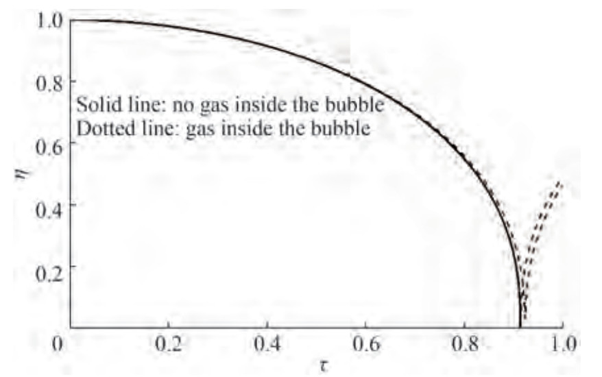 Figure 1 Dynamics of vapor bubbles in the absence (solid line) and presence of the gas (dotted line)
The results presented in Figure 1 reveal that in the absence of gas (δg = 0), the bubble eventually collapses, and further expansion does not occur. By contrast, a tendency for bubble expansion is observed in the presence of gas in the bubble (δg ≠ 0), which further develops into undamped oscillations.
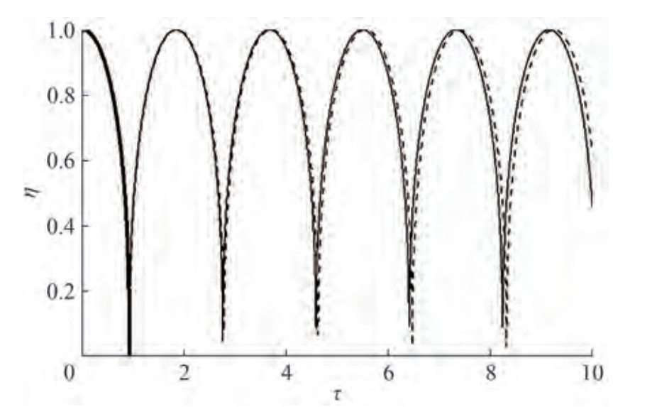 Figure 2 Undamped oscillations of the bubble in the presence of gas (thick solid line: δg = 0 indicates the absence of gas, the solid line indicates δg = 0.01, and the dotted line indicates δg = 0.001)
Capillarity and viscosity are considered, which can be conducted by including two additional terms into the Rayleigh-Plesset equation (Miniovich et al. 1972):
$$ \eta \ddot{\eta}+\frac{3}{2} \dot{\eta}^2-\delta_g \eta^{-3 \gamma}+\frac{2 D}{\eta}+\frac{C \dot{\eta}}{\eta}+1=0 $$ (21) where parameters D and C are respectively expressed through the coefficients of dynamic viscosity μ and surface tension σ of the fluid
$$ C=\frac{\mu}{R_0 \sqrt{P_0 \rho_0}}, D=\frac{\sigma}{R_0 P_0} $$ (22) For the first-order estimation: R0=10−5 m, P0≃105 N/m2, for water temperature of 10 ℃, μ =133.1×10⁻⁵ kgf·s·m−2; thus, С ≃ 0.013 3 and D = 0.073 5 can be obtained.
Figure 3 shows the data calculation of the bubble radius versus time for gas content fraction δg = 0.001 and considering the viscosity and surface tension of the fluid (C = 0.013 3; D = 0.073 5).
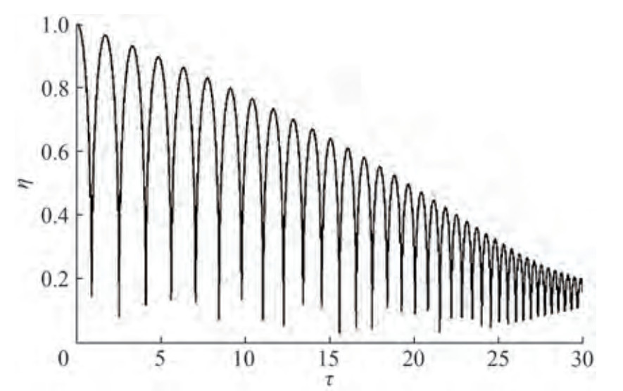 Figure 3 Damped oscillations of gas-containing bubbles considering the capillarity and viscosity of the fluid (δg = 0.001, R0=10−5 m)
Notably, the bubble executes damped oscillations due to fluid viscosity. Considering Equation (21) prompts the analytical integration for С = 0. Using the previously discussed approach, the following is written:
$$ \eta \frac{\mathrm{d} \dot{\eta}^2}{\mathrm{~d} \eta}+3 \dot{\eta}^2-2 \delta_g \eta^{-3 \gamma}+\frac{4 D}{\eta}+2=0 $$ (23) Equation (23) is linear considering the function $ \dot{\eta}^2$; thus, its general solution can be represented as
$$ \dot{\eta}^2=K \eta^{-3}-\frac{2}{3}-\frac{2}{3} \frac{\delta_g}{\gamma-1} \eta^{-3 \gamma}-\frac{2 D}{\eta} $$ (24) where the first term is a homogeneous solution of Equation (23) and other terms satisfy this equation, which can be verified by substitution. The constant K is determined by applying the following initial condition: $ \dot{\eta}$(1) = 0, which gives
$$ K=\frac{2}{3}\left(1+\frac{\delta_g}{\gamma-1}\right)+2 D $$ (25) Substituting this value of K, another value (other than one) of η = ηmin, which corresponds to the minimal radius of the bubble surface tension, can be derived. Integrating (24) considering time over the interval η ∈ [ηmin, 1], the time necessary to reach the minimum radius for a gas-containing bubble considering capillarity is identified.
Some calculation results obtained through direct numerical integration of Equation (21) without considering the gas contents (δg = 0) are given in Figure 4. In this figure, where the dotted lines above the solid line correspond to the influence of viscosity without capillarity (С ≠ 0, D = 0), while those under the solid line correspond to the influence of capillarity without viscosity (С = 0, D ≠ 0)Thus, surface tension reduces the period of bubble collapse, and viscosity increases such a period based on Figure 4.
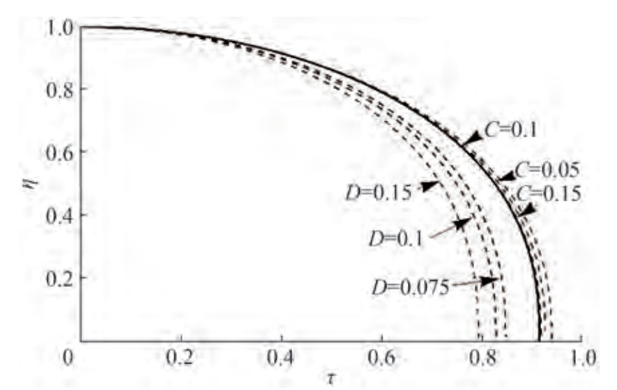 Figure 4 Influence of viscosity and capillarity on bubble dynamics under compression with no gas inside (dotted line) (the solid line corresponds to the compression curve for the bubble with no influence of viscosity and capillarity)
4 Case of a bubble motion in gradient pressure field near the rounded leading edge of a foil
Known mathematical emulators of pressure gradient for studying vapor bubble response are based on certain plausible laws of variation of the external pressure. The simplest law is the case of an instantaneous stepped growth in pressure, which has been previously referred to in this paper. The following proposed model of a flow near the rounded leading edge of a hydrofoil represents a natural mathematical testbed, which can generate growth and pressure drop. In this model, parameters characterize the geometry and kinematics of the foil. To investigate the dynamics and acoustics of the bubble, the (outer) flow description for a foil of a given configuration should first be constructed. Then, the local (inner) flow near a rounded leading edge should be comprehensively considered. Finally, the dynamics of a bubble moving along a selected streamline, thus becoming subject to the action of the pressure gradients, should be observed using the Rayleigh-Plesset equation. The leading edge flow is characterized by a large curvature of the streamlines, which depend on the relative thickness δ, relative camber δc, and angle of attack α (in radians) of the foil. All these nondimensional parameters are considered in the order of δ, whereas δ → 0. Note that, practically, relative thickness, camber and angle of attack (in radians) of foils and blades tend to be quite small. The division of the flow field into outer and inner regions according to characteristic scales to solve the problem of the flow past a foil using the MAE method is illustrated in Figure 5.
 Figure 5 Division of the flow field around a foil (MAE)
To obtain a solution for the flow around the foil using the MAE method, the outer flow problem, in which (x, y) = O(1), δ → 0, should first be considered.
4.1 Outer flow field
In the outer limit, the foil degenerates into a slit x ∈(−1, 1), y=0 ± 0. The application of linear theory (Rozhdestvensky 1979) indicates that relative flow velocity on the contour of a thin and slightly curved foil in a steady incompressible ideal fluid flow can be obtained in the form
$$ \begin{gathered} v^o(x)=1+\frac{\delta}{{\rm{ \mathsf{ π} }}} \mathrm{v} . \mathrm{p} . \int\limits_{-1}^1 \frac{f_t^{\prime}(\xi) \mathrm{d} \xi}{x-\xi} \\ \pm \frac{\delta}{{\rm{ \mathsf{ π} }}} \sqrt{\frac{1-x}{1+x}} \text { v.p. } \int\limits_{-1}^1 \frac{\bar{\delta}_c f_c^{\prime}(\xi)-\bar{\alpha}}{x-\xi} \sqrt{\frac{1+\xi}{1-\xi}} \mathrm{d} \xi \end{gathered} $$ (26) where υo is the velocity on the upper (sign «+») and lower (sign «-») sides of the foil, which is related to the speed of flow in upstream infinity U0; δ is the relative thickness of the foil, δc is the relative camber of the foil, and δc is the angle of attack in radians. ft (x) and fc (x) are functions of the order of O(1), respectively describing distributions of thickness and curvature; α = α/δ, δc = δc /δ are parameters of the order of O(1).
Notably, the integrals in (26) are defined on the basis of the Cauchy principal value and can be reduced to quadrature for practically any foil with an analytical description. A table of necessary integrals, which covers classical families of foils, can be found in the section "Airfoil Integrals" of Appendix B, NACA TN 3390 (Van-Dyke 1955). The solutions, which are expressed by the formula (26), lose validity at distances of the order O(δ2) from the rounded leading edge. In particular, the velocity and linearized pressure have a square-root singularity at the leading edge.
4.2 Inner flow field
To investigate the flow pattern near the leading edge thoroughly, the inner description of the flow problem should be discussed by introducing stretched local coordinates X = (1 + x) /rle, Y = y/rle, Z = X + iY.
For any analytical foil with the rounded leading edge, the latter can be approximated by an osculating parabola with an asymptotic error of O(δ2). For example, in the case of elliptical foil with a thickness function ft (x) = $ \sqrt{1-x^2}$ the vicinity of the leading edge (xle = 1 + x, X = xle /δ2) can be identified on the basis of the following approximation of the stretched foil contour
$$ \begin{gathered} Y=\frac{y_{\mathrm{le}}}{\delta^2}=\pm \frac{\delta f_t}{\delta^2}=\pm \frac{\delta \sqrt{x_{\mathrm{le}}\left(2-x_{\mathrm{le}}\right)}}{\delta^2}= \\ \pm \frac{\delta \sqrt{\delta^2 X\left(2-\delta^2 X\right)}}{\delta^2} \approx \pm \sqrt{2 X}+O\left(\delta^2\right) \end{gathered} $$ (27) The following can be obtained for foils of general form with a rounded leading edge:
$$ Y=\pm \sqrt{2 \bar{r}_{\mathrm{le}} X}+O\left(\delta^2\right) $$ (28) For example, the thickness distribution of NACA fourdigit sections is given by the following equation (Abbot and Von Doenhoff 1959) and rewritten with x1 = (1 + x) /2
$$ \begin{aligned} \pm f_t\left(x_1\right)=& 1.4845 \sqrt{x_1}-0.6300 x_1-1.7580 x_1^2+\\ & 1.4215 x_1^3-0.5075 x_1^4 \end{aligned} $$ (29) The thickness functions of the modified NACA four-digit and five-digit series wing sections ahead of the maximum thickness position are defined by the following equation:
$$ \pm f_t\left(x_1\right)=a_0 \sqrt{x_1}+a_1 x_1+a_2 x_1^2+a_3 x_1^3 $$ (30) Introducing stretched X = x1 /δ2 and comparing (28) and (30), the radius of curvature of the rounded leading edge for the NACA four-digit and five-digit series is equal to
$$ r_{\mathrm{le}}=\delta^2 a_0^2 / 2 $$ (31) The complex potential of the flow near a leading rounded edge, which has an asymptotic error of O(δ2) as shown above and is approximated by an osculating semi-infinite parabola, can be easily constructed by the methods of the theory of complex variable (Rozhdestvensky 1979).
The inner flowfield can be constructed by superposition of a local symmetrical flow (a) and a local circulatory flow (b) past an osculating parabola. A symmetrical flow past osculating parabola with a unit incoming uniform flow velocity is readily constructed via conformal mapping of the domain external to the parabola onto the auxiliary upper plane $ w_a=Z-\bar{r}_{\mathrm{le}}-\mathrm{i} \sqrt{2 \bar{r}_{\mathrm{le}} Z-\bar{r}_{\mathrm{le}}^2}$ (where Z = X + iY). This complex function wa represents the complex potential of the flow under study. Taking derivative considering Zyields a complex conjugate velocity
$$ \frac{\mathrm{d} w_a}{\mathrm{~d} Z}=1-\frac{\mathrm{i} \cdot \bar{r}_{\mathrm{le}}}{\sqrt{2 \bar{r}_{\mathrm{le}} Z-\bar{r}_{\mathrm{le}}^2}} $$ (32) the module of which represents full velocity on the parabola contour due to symmetrical flow through the following expression:
$$ v_a(X)=\left|\frac{\mathrm{d} w_a}{\mathrm{~d} Z}\right|=\sqrt{\frac{X}{X+\bar{r}_{\mathrm{le}} / 2}} $$ (33) Therefore, the critical point associated with symmetrical flow coincides with the origin of the coordinate system.
The circulatory (asymmetrical) part of the flow is then discussed. A circulatory flow generally occurs around the parabolic leading edge, resulting in the critical point displacement. This circumstance can be accounted for by considering a component of the local flow, which is asymmetrical considering the Xaxis (circulatory flow past parabola with the unit speed at a point Z = 0).
Notably, the function $ f_b=\sqrt{Z-\bar{r}_{\mathrm{le}} / 2}$ conformally maps the domain external to the parabola onto a semiplane $ \operatorname{Im} f_b>\sqrt{\bar{r}_{\mathrm{le}} / 2}$. The flow in this auxiliary plane represents a uniform flow with complex potential wb = Cb · fb. To determine the constant Cb the magnitude of the velocity in the physical plane at Z = 0 is assumed to be equal to one, resulting in the following expression for full velocity on the parabola contour due to circulatory (asymmetrical) flow.
$$ v_b=\left|\frac{\mathrm{d} w_b}{\mathrm{~d} Z}\right|=\frac{\sqrt{\bar{r}_{\mathrm{le}}}}{\sqrt{2 X+\bar{r}_{\mathrm{le}}}} $$ (34) Summing up the symmetrical and circulatory flow velocities on the parabola contour, the following expression for full velocity on the contour of the parabolic leading edge (osculating parabola) is concluded as follows:
$$ v^i(X)=\sqrt{\frac{X}{X+\frac{1}{2} \bar{r}_{\mathrm{le}}}}\left(U_1 \pm \frac{U_2}{\sqrt{X}}\right) $$ (35) where plus and minus respectively correspond to the upper part of the contour and the lower part of the parabola contour.
Figure 6 shows the flow patterns associated with symmetrical (a) and asymmetrical (b) flows around the parabolic leading edge. Figure 7 shows the pattern of the inner (local flow) around the parabolic leading edge formed as a superposition of symmetric and asymmetric flow patterns.
 Figure 6 Typical patterns of streamlines
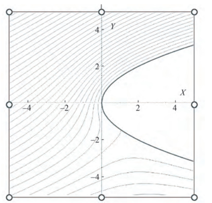 Figure 7 Typical pattern of the local flow around the parabolic leading edge containing stagnation line (in stretched coordinates X and Y)
Parameters U1 and U2 are unknown and should be determined through asymptotic matching with the outer description of the flow velocity. Matching the two-term outer expansion (26) of the velocity on the parabola with the twoterm inner expansion (35) of the velocity on the parabola yields
$$ {U_1} = 1 + \frac{\delta }{{\rm{ \mathsf{ π} }}}\mathop {\lim }\limits_{x \to - 1} {\rm{ v}}{\rm{.p}}{\rm{. }}\int\limits_{ - 1}^1 {\frac{{f_t^\prime (\xi){\rm{d}}\xi }}{{x - \xi }}} = 1 + \delta \cdot {u_\delta } $$ (36) $$ \begin{array}{c} {U_2} = \frac{{\sqrt 2 }}{{\rm{ \mathsf{ π} }}}\mathop {\lim }\limits_{x \to - 1} {\rm{ v}}{\rm{.p}}{\rm{. }}\int\limits_{ - 1}^1 {\frac{{{{\bar \delta }_c}f_c^\prime (\xi) - \bar \alpha }}{{x - \xi }}} \sqrt {\frac{{1 + \xi }}{{1 - \xi }}} {\rm{d}}\xi = \\ \bar \alpha \sqrt 2 + \frac{{{{\bar \delta }_c}\sqrt 2 }}{{\rm{ \mathsf{ π} }}}\mathop {\lim }\limits_{x \to - 1} {\rm{ v}}{\rm{.p}}{\rm{.}}\int\limits_{ - 1}^1 {\frac{{f_c^\prime (\xi)}}{{x - \xi }}} {\rm{ }}\sqrt {\frac{{1 + \xi }}{{1 - \xi }}} {\rm{d}}\xi = \\ \bar \alpha \sqrt 2 + {{\bar \delta }_c} \cdot {u_c} \end{array} $$ (37) Complex potentials and conjugate velocities of these flows can be easily derived following Rozhdestvensky (1979).
Relative full velocity on the contour of the parabolic leading edge (osculating parabola) can be obtained using (35): where υi is a full velocity at a point of the parabolic contour on its upper (sign «+») and lower (sign «-») sides; X = xle/rle is the stretched abscissa, which is measured from the apex of the edge; rle = rle /δ2, where rle is the radius of curvature of the leading edge, which is related to halfchord of the foil; U1 and U2 are parameters associated correspondingly with relative velocities of the local flow, coming upon the edge, and circulatory flow, which is tangential to the contour of the edge.
Notably, for a given family of analytical foils, the ratio of the nondimensional leading edge radius to the square of relative thickness rle is a constant.
The pressure coefficient at points of the leading edge contour considering (27) can be calculated using the following formula:
$$ p^i(X)=1-\frac{X}{X+\frac{1}{2} \bar{r}_{\mathrm{le}}}\left(U_1 \pm \frac{U_2}{\sqrt{X}}\right)^2 $$ (38) As shown in Rozhdestvensky (1979), parameters U1 and U2 can be obtained through asymptotic matching (smooth connecting) of the outer solution (26) and inner solution describing the flow near the osculating parabola (35). Notably, using formulas (35) and (38) implies that the bubble under investigation moves along the streamline, coinciding with the contour of the leading edge. Corresponding values of the stream function must be employed to treat bubble movement along other streamlines.
4.3 Asymptotic matching
In particular, in the case of steady flow past an analytical foil these parameters have the following structure:
$$ U_1=1+\delta u_\delta $$ (39) $$ U_2=\bar{\alpha} \sqrt{2}-\bar{\delta}_c u_c $$ (40) where uδ and uc depend entirely on the foil geometry and respectively follow (36) and (37) as
$$ {u_\delta } = \frac{1}{{\rm{ \mathsf{ π} }}}\mathop {\lim }\limits_{x \to - 1} {\rm{v}}{\rm{.p}}{\rm{.}}\int\limits_{ - 1}^1 {\frac{{f_t^\prime (\xi){\rm{d}}\xi }}{{x - \xi }}} $$ (41) $$ {u_c} = \frac{{\sqrt 2 }}{{\rm{ \mathsf{ π} }}}\mathop {\lim }\limits_{x \to - 1} {\rm{v}}{\rm{.p}}{\rm{.}}\int\limits_{ - 1}^1 {\frac{{f_c^\prime (\xi)}}{{x - \xi }}} \sqrt {\frac{{1 + \xi }}{{1 - \xi }}} {\rm{d}}\xi $$ (42) Table 2 presents the numerical values for uδ, uc and rle for some foil families (for example, Abbott and Von Doenhoff (1959)).
Table 2 Values uδ, uc and rle for different foil familiesFoil type uδ uc rle Ellipse 1 0 1 NACA 66012 0.817 0 0.874 Gö (Walchner foil) 0.919 0.246 0.964 NACA4412 2 0.296 1.026 NACA66 m (a = 0.8) 0.75 0.208 0.848 Zhukovsky foil 2.288 0 2.35 The closed form of the expressions for relative velocity and pressure coefficient on the contour of semi-infinite osculating parabola, which coincides with the contour of the rounded leading edge, enables the acquisition of simple and universal formulas for the minimum magnitude of pressure coefficient and abscissas of critical point (pi = 1) and the point of minimal pressure (pi = pmini).
Equating to zero the derivative of the pressure coefficient pi (X) considering stretched abscissa X, yields the following expression for stretched abscissa of the minimum pressure point:
$$ X_m=\frac{\left(x_{\mathrm{le}}\right)_m}{r_{\mathrm{le}}}=\frac{\left(x_{\mathrm{le}}\right)_m}{\delta^2 \bar{r}_{\mathrm{le}}}=\frac{U_1^2}{4 U_2^2} $$ (43) where (xle)m represents the abscissa of the minimum pressure, which is related to the half-chord of the foil.
4.4 Minimum pressure coefficient
Substituting (43) into (38) leads to the following expression for the minimum magnitude of the pressure coefficient:
$$ p_{\min }^i=1-U_1^2-\frac{2 U_2^2}{\bar{r}_{\mathrm{le}}} $$ (44) The expression (35) for the velocity on the contour of the leading edge reveals that this velocity is equal to zero on the lower side of the foil at a (critical) point with stretched abscissa:
$$ X_s=\frac{\left(x_{\mathrm{le}}\right)_s}{\delta^2 \bar{r}_{\mathrm{le}}}=\left(\frac{U_2}{U_1}\right)^2 $$ (45) Considering expressions (41) and (43) leads to the following formulas (Rozhdestvensky 1979):
$$ X_m X_s=\frac{1}{4} \bar{r}_{\mathrm{le}}^2 $$ (46) $$ \left(x_{\mathrm{le}}\right)_m \cdot\left(x_{\mathrm{le}}\right)_s=\frac{1}{4} r_{\mathrm{le}}^2 $$ (47) The product of the stretched abscissas of the critical point and the point of pressure minimum for a given family of analytical foil is a constant according to (46).
In the simplest case of elliptic foil of relative thickness δ, streamlined at an angle α, the expression for minimal pressure coefficient and stretched abscissas of the points of minimum and maximum pressure takes the form
$$ p_{\min }^i(\alpha, \delta) =1-(1+\delta)^2-4 \frac{\alpha^2}{\delta^2} $$ (48) or
$$ p_{\min }^i(\alpha, \delta) =-2 \delta-\delta^2-4 \frac{\alpha^2}{\delta^2} $$ (49) $$ X_s =\frac{2 \alpha^2}{\delta^2(1+\delta)^2} $$ (50) $$ X_m =\frac{(1+\delta)^2 \delta^2}{8 \alpha^2} $$ (51) 4.5 Examples of pressure distributions near the leading edge
Shown below in the Figures 8‒11 are typical nondimensional pressure distributions near the rounded leading edge exemplified for different foil families. Notably, these pressure graphs are plotted as function of the stretched abscissa of the foil measured from the apex of the osculating parabola, or versus stretched arc coordinate measured from the flow stagnation point.
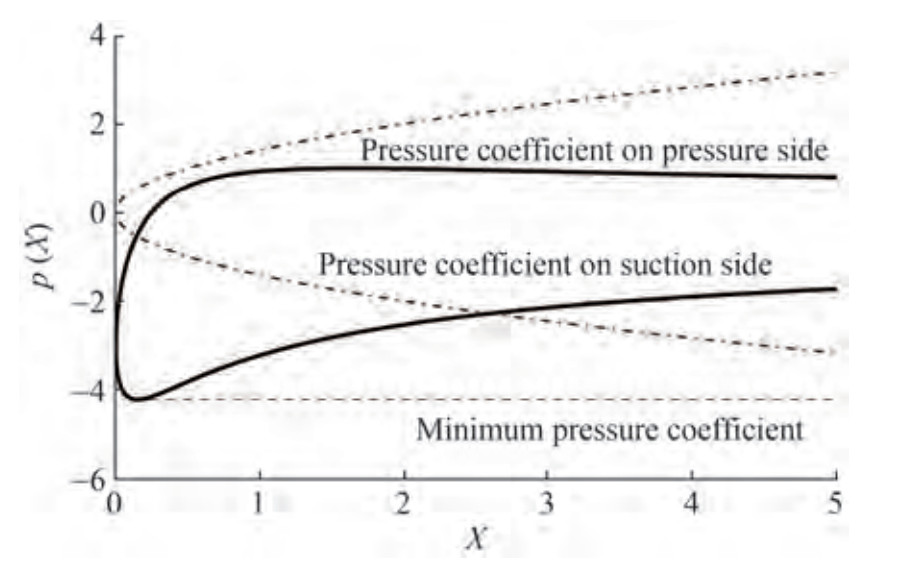 Figure 8 Distribution of pressure coefficient along the leading edge of the foil versus stretched abscissa X (ellipse, α = δ = 0.1)
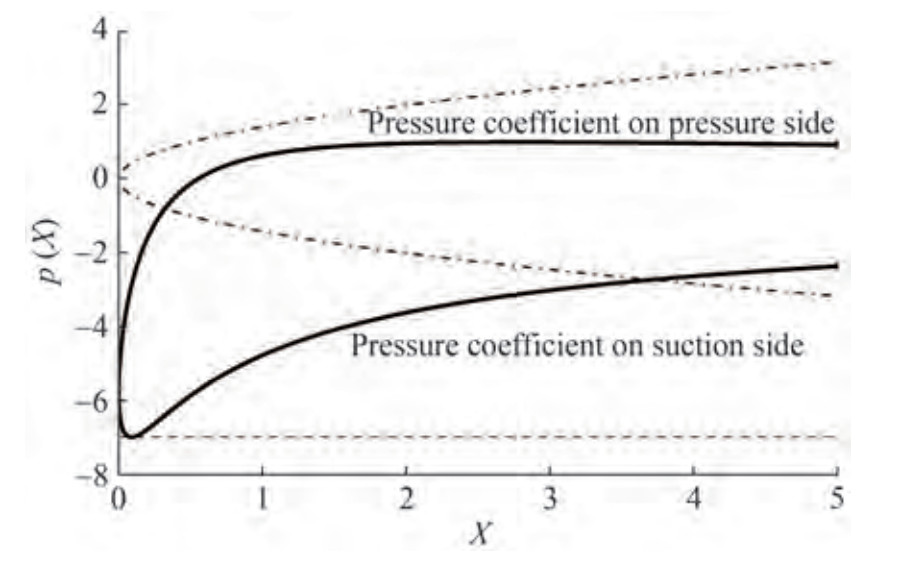 Figure 9 Distribution of pressure coefficient along the leading edge of the foil versus stretched abscissa X (ellipse α =0.13, δ = 0.1)
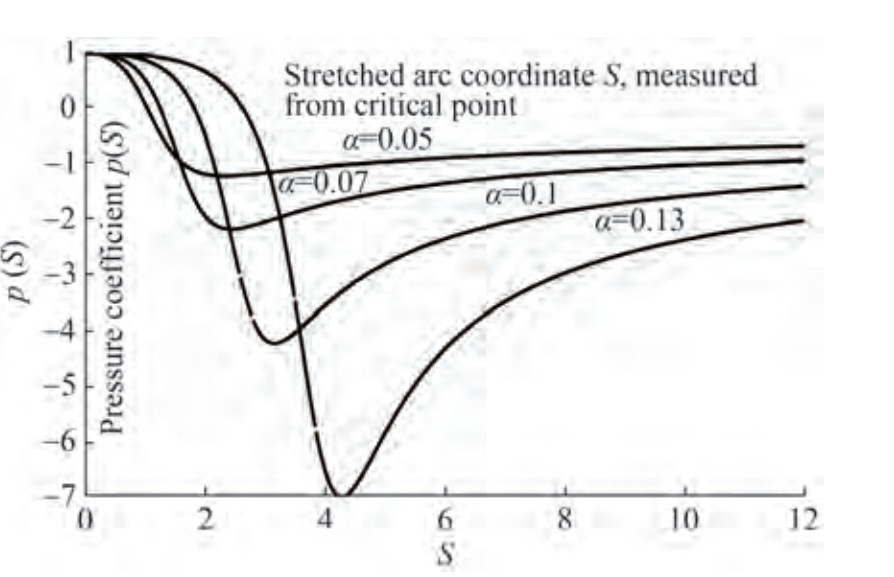 Figure 10 Dependence of pressure coefficient on the stretched arc coordinate, measured from the critical point (ellipse, δ = 0.1)
 Figure 11 Distribution of pressure coefficient along the leading edge of the elliptical; NACA66 m and Zhukovsky foil versus stretched abscissa X (δ = 0.1, α = 0.13)
Figure 11 shows the calculated pressure distributions on the parabolic leading edge of different foils for α = 0.13; δ = 0.1.
4.6 Prediction of bubble dynamics near the rouded leading edge using the Raileigh-Plesset equation
A simplified (without account of surface tension, viscosity, and gas content) form of the Rayleigh-Plesset equation is used to model the dynamics of the (vapor) cavitation bubble near the rounded leading edge of the foil (Rayleigh 1917; Brennen 1995)
$$ R \ddot{R}+\frac{3}{2} \dot{R}^2=-\frac{P(t)}{\rho} $$ (52) where R = R(t) is the bubble radius in m, t is the time in s, P(t) is the pressure outside of the bubble in N/m2 as a function of time, ρ is the density of the fluid in kg/m3, and dots denote differentiation in time. To solve this equation, the following initial conditions will be considered:
$$ R(0)=R_0, \dot{R}(0)=0 $$ (53) The vapor bubble, which appeared at a certain point of the flow, is assumed to continue its movement along a streamline passing through this point to obtain the dependence of pressure P(t) on time. The current work is limited by the case when the bubble is moving along the streamline adjacent to the foil contour.
Dimensional pressure P is expressed through pressure coefficient p by using the formula
$$ P=p \frac{\rho U_0^2}{2}+P_0 $$ (54) where P0 is pressure at infinity, U0 is the velocity of the oncoming flow, and p is the pressure coefficient. Notably, the flow velocity, in which a vapor bubble occurs at a certain point of the foil contour, is equal to the speed of cavitation inception U0ci, which, in turn, is determined using the following formula:
$$ U_0^{\mathrm{ci}}=\sqrt{\frac{2\left(P_0-P_{s v}\right)}{\rho \kappa}} $$ (55) where Psv is the pressure of saturated vapor and κ is the cavitation number.
From the viewpoint of calculated data representation on bubble dynamics, rendering the Rayleigh-Plesset Equation (52) to nondimensional form is convenient.
Nondimensional time is introduced as follows:
$$ \tau=\frac{t}{R_0} \sqrt{\frac{P_0}{\rho}} $$ (56) Using the formulas presented earlier, determining the parametric dependences of nondimensional time τ and pressure coefficient p on stretched abscissa X is easy. As previously mentioned, the vapor bubble is assumed to move along the streamline coinciding with the foil contour streamline. Considering the differential equation of bubble motion along the streamline as a material point, the following can be written:
$$ \begin{aligned} &v^i(S)=\frac{c}{U_0^{\text {ci }}} \frac{\mathrm{d} s}{\mathrm{~d} t}=\frac{\delta^2 \bar{r}_{\mathrm{le}}}{U_0^{\mathrm{ci}} R_0} \sqrt{\frac{P_0}{\rho}} \frac{\mathrm{d} S}{\mathrm{~d} \tau}=\\ &\frac{r_{\mathrm{le}}}{U_0^{\mathrm{ci}} R_0} \sqrt{\frac{P_0}{\rho}} \frac{\mathrm{d} S}{\mathrm{~d} \tau}=\frac{r_{\mathrm{le}}}{R_0} \sqrt{\frac{\kappa}{2}\left(1-\frac{P_{\mathrm{sv}}}{P_0}\right)} \frac{\mathrm{d} S}{\mathrm{~d} \tau} \end{aligned} $$ (57) where S = s/rle, s and S are the arc coordinates of the bubble center, which is measured from the critical point. Notably, the pressure of saturated vapor Psv is substantially less than P0. Therefore, (20) can be rewritten in compact form as follows:
$$ v^i(S)=\frac{r_{\mathrm{le}}}{R_0} \sqrt{\frac{\kappa}{2}} \frac{\mathrm{d} S}{\mathrm{~d} \tau} $$ (58) Notably, the equations of the suction (+) and pressure (−) sides for a parabolic leading edge are
$$ Y(X)=\pm \sqrt{2 X} $$ (59) The relationship of the arc coordinate S and abscissa X for the elliptical foil is defined by the expression
$$ \frac{\mathrm{d} S}{\mathrm{~d} X}=\pm \sqrt{1+\left(\frac{\mathrm{d} Y}{\mathrm{~d} X}\right)^2}=\pm \sqrt{1+\left(\frac{1}{\sqrt{2 X}}\right)^2}=\pm \sqrt{\frac{X+\frac{1}{2}}{X}} $$ (60) Integrating the point of inception of vapor bubble (with stretched abscissa Xci) helps obtain the relationship of the stretched arc coordinate and abscissa in the following form:
$$ \begin{gathered} S=\pm \int\limits_{X_{\mathrm{ci}}}^X \sqrt{\frac{X+\frac{1}{2}}{X}} \mathrm{~d} X= \\ \pm\left(\sqrt{X} \sqrt{X+\frac{1}{2}}-\sqrt{X_{\mathrm{ci}}} \sqrt{X_{\mathrm{ci}}+\frac{1}{2}}\right. \\ \left.+\frac{1}{2} \ln \frac{\sqrt{X}+\sqrt{X+1}}{\sqrt{X_{\mathrm{ci}}}+\sqrt{X_{\mathrm{ci}}+1}}\right) \end{gathered} $$ (61) Therefore, the stretched abscissa Xci of the foil contour point where the bubble originated can be determined using the Eq. (38) from the equation below:
$$ p\left(X_{\mathrm{ci}}\right)=-\kappa $$ (62) In particular, if the bubble emerged at the point of minimal pressure, then
$$ X_{\mathrm{ci}}=X_m, p\left(X_{\mathrm{ci}}\right)=p\left(X_m\right)=p_{\min }=-\kappa $$ (63) The dependence of nondimensional time τ on X can be found after the integration of Equation (20) in the form
$$ \begin{array}{*{20}{c}} {\tau = \frac{{{r_{{\rm{le}}}}}}{{{R_0}}}\sqrt {\frac{\kappa }{2}} \int\limits_0^S {\frac{{{\rm{d}}S}}{{{\upsilon ^i}(S)}}} = \frac{{{r_{{\rm{le}}}}}}{{{R_0}}}\sqrt {\frac{\kappa }{2}} \int\limits_{{X_{{\rm{ci}}}}}^X {\frac{{\frac{{{\rm{d}}S}}{{{\rm{d}}X}}{\rm{d}}X}}{{{\upsilon ^i}\left( X \right)}}} }\\ { \pm \frac{{{r_{{\rm{le}}}}}}{{{R_0}}}\sqrt {\frac{\kappa }{2}} \int\limits_{{X_{{\rm{ci}}}}}^X {\frac{{\left( {X + \frac{1}{2}} \right){\rm{d}}X}}{{\sqrt X \left( {{U_1}\sqrt X \pm {U_2}} \right)}}} = }\\ { \pm \frac{{{r_{{\rm{le}}}}}}{{{R_0}}}\sqrt {\frac{\kappa }{2}} \left\{ {\frac{1}{{U_1^2}}\left[ {2{U_1}\left( {\sqrt {{X_{{\rm{ci}}}}} - \sqrt X } \right) + {U_1}\left( {X - {X_{{\rm{ci}}}}} \right)} \right]} \right.}\\ {\left. { + \frac{1}{{{U_1}}}\left( {1 + 2\frac{{U_2^2}}{{U_1^2}}} \right)\ln \frac{{{U_1}\sqrt X \pm {U_2}}}{{{U_1}\sqrt {{X_{{\rm{ci}}}}} \pm {U_2}}}} \right\}} \end{array} $$ (64) Eqs. (38) and (64) provide parametric dependence p[X(τ)]. Finally, the dependence of dimensional pressure on the nondimensional time takes the form
$$ \begin{aligned} &P(\tau)=\frac{p(\tau)}{\kappa}\left(P_0-P_{\mathrm{sv}}\right)+P_0 \\ &=P_0\left[1+\frac{p(\tau)}{\kappa}\left(1-\frac{P_{\mathrm{sv}}}{P_0}\right)\right] \end{aligned} $$ (65) After normalization of the bubble radius R by its magnitude at the moment of inception R0, the Rayleigh-Plesset equation can be written in the following (nondimensional) form:
$$ \eta \frac{\mathrm{d}^2 \eta}{\mathrm{d} \tau^2}+\frac{3}{2}\left(\frac{\mathrm{d} \eta}{\mathrm{d} \tau}\right)^2=-1-\frac{p(\tau)}{\kappa}\left(1-\frac{P_{\mathrm{sv}}}{P_0}\right) $$ (66) where η = R(τ) = R(τ) /R0. Such a form of the Rayleigh-Plesset equation allows the compact presentation of calculated data. Some calculated results are shown below. In particular, Figure 12 shows that when cavitation occurs on the foil suction side at the minimum pressure point, a dependence of normalized bubble radius η = R on nondimensional time τ is observed for an elliptical foil with relative thickness δ = 0.1 for different values of angle of attack (in radians) and the ratio of the initial radius of the bubble to the radius of curvature of the leading edge R0 /rle = 0.2.
 Figure 12 Typical dependences of normalized radii of vapor bubbles on the nondimensional time for different magnitudes of the angle of attack and elliptical foil, δ = 0.1, R0 /rle = 0.2
 Figure 13 Dependences of nondimensional time at which the bubble collapses on the ratio of the angle of attack (in radians) to the relative thickness of the foil for (κ = − pmin; δ = 0.1; R0 /rle = 0.2)
Figures 14 and 15 show the typical calculated data on vapor bubble dynamics for values of cavitation number κ < − pmin. In this case, after its origination, the bubble first gets into a low-pressure zone and inflates. Then, is compressed until its collapse after entering into an increased pressure zone. The right-hand side of Equation (66) is denoted on the same graphs by dashed lines.
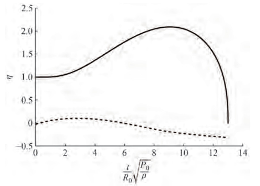 Figure 14 Bubble dynamics at κ < −pmin, κ = 3, δ = 0.1, α = 0.1, pmin = − 4.21, R0/rle = 0.2
 Figure 15 Bubble dynamics at κ < −pmin, κ = 0.96, δ = 0.1, α = 0.07, pmin=−2.17, R0/rle = 0.2
 Figure 16 Dependences of normalized radii of vapor bubbles on nondimensional time for different foils, α = 0.13, δ = 0.1, R0 /rle = 0.2
5 Calculation of acoustic pressure and spectral characteristics of contraction/collapse of a vapor bubble
The most intense and occasionally catastrophic consequences of the collapse of the bubbles are the noise produced by the impulse pressures accompanying its compression and the erosion of the body surface material. To the leading approximation, the acoustic pressure is represented by the term accounting for the bubble volume variation. The variable acoustic (dimensional) pressure in the far field is given by the following formula:
$$ \begin{aligned} p_a=& \frac{\rho}{4 {\rm{ \mathsf{ π} }} r} \cdot \frac{\mathrm{d}^2 V(t)}{\mathrm{d} t^2}=\frac{\rho}{3 r} \frac{\mathrm{d}^2}{\mathrm{~d} t^2} R^3(t)=\\ & \frac{\rho}{r}\left(2 R \dot{R}^2+3 R^2 \ddot{R}\right) \end{aligned} $$ (67) where r is the distance between the center of the bubble and the point of measurement, and the "dots" denote differentiation considering dimensional time t. Regarding nondimensional values, considering the notations introduced earlier, (55) can be written as
$$ p_a=\frac{R_0 P_0}{r}\left(2 \eta \dot{\eta}^2+\eta^2 \ddot{\eta}\right) $$ (68) where the "dots" denote differentiation considering nondimensional time τ. The nondimensional acoustic pressure is introduced as follows:
$$ \bar{p}_a=\frac{R_0}{r}\left(2 \eta \dot{\eta}^2+\eta^2 \ddot{\eta}\right)=\frac{R_0}{r} \tilde{p}_a(\tau) $$ (69) where $ \tilde{p}_a$(τ) is a nondimensional function, which characterizes the dependence of the acoustic pressure on nondimensional time. The calculation of spectral characteristics of the acoustic signal accompanying the collapse of the bubble generally requires applying the integral Fourier transform to the pressure as a function of time. In particular, this procedure allows for determining the frequency ranges where the acoustic signal energy is concentrated. The calculated data presented below show that the prevailing intensity of the acoustic signal at the stage of bubble compression is observed near the moment of its collapse. Herein, to the leading approximation, the acoustic pressure impulse can be treated as a triangular one to simplify the spectrum analysis. The signal spectrum in dimensional terms can be written down as follows:
$$ |S(\mathrm{i} \omega)|=\frac{p_a^{\max } \Delta t_s}{2}\left[\frac{\sin \left(\omega \Delta t_s / 4\right)}{\omega \Delta t_s / 4}\right]^2 $$ (70) where S(iω) is the complex spectrum of the triangular signal, ω is the circular frequency of a concrete harmonic in s−1, Δts is the interval of action of the triangular impulse, and pamax is the peak value of the triangular impulse. Furthermore, for convenience of recalculation of characteristics and in accordance with similarity theory, nondimensional magnitudes are presented as follows:
$$ |\bar{S}(\mathrm{i} \bar{\omega})|=\frac{r}{R_0^2 \sqrt{P_0 \rho}}|S(\mathrm{i} \omega)|=\frac{\tilde{p}_a^{\max } \Delta \tau_s}{2}\left[\frac{\sin \left(\bar{\omega} \Delta \tau_s / 4\right)}{\bar{\omega} \Delta \tau_s / 4}\right]^2 $$ (71) The following denotations in Eq. (71) represent the signal spectrum in a nondimensional form: pamax is the nondimensional peak value of the triangular impulse, ω is the nondimensional circular frequency of a concrete harmonic, Δτs is the nondimensional time interval of action of the triangular impulse. The factor in front of the expression (71) represents a nondimensional area of the triangular impulse equal to
$$ \sigma_{\Delta}=\frac{\tilde{p}_a^{\max } \Delta \tau_s}{2} $$ (72) The characteristics of acoustic impulse accompanying the collapse of gas-containing bubbles in concrete cases of external pressure growth are considered.
5.1 Sudden increase in pressure
Figure 17 reflects the dependence of nondimensional acoustic pressure versus nondimensional time for gas content fraction δ = 0.001. In this case, the maximum value of nondimensional acoustic pressure is equal to $ \tilde{p}_a^{\max }$ = 462.5, and the nondimensional impulse area is obtained by integrating the function $ \tilde{p}_a $(τ) across the interval τ ∈[0.90, 0.93] and is equal to σΔ = 0.8. Therefore, the nondimensional time interval of action of the area-equivalent triangular impulse is Δτs = 2σΔ /$ \tilde{p}_a^{\max }$ = 0.003 46.
 Figure 17 Nondimensional acoustic pressure versus nondimensional time (during the period of compression and near the moment of the bubble collapse)
The nondimensional spectrum of this signal is shown below.
 Figure 18 Spectrum of acoustic pressure impulse during the collapse of gas-containing bubbles for the case of instantaneous pressure increase
5.2 Compression of a bubble moving along the contour of the rounded leading edge of a thin, slightly curved hydrofoil at a small angle of attack
Time functions of the radius of the contracting vapor bubble at various angles of attack α (in radians) were obtained for the case of a thin elliptic hydrofoil with relative thickness δ. The presence of some quantity of gas, which is represented by gas fraction δg should be considered to evaluate the acoustic characteristics of the bubble collapse in this case. Therefore, Eq. (66) is rewritten as follows:
$$ \eta \ddot{\eta}+\frac{3}{2} \dot{\eta}^2-\delta_g \eta^{-3 \gamma}+1+\frac{p(\tau)}{\kappa}\left(1-\frac{P_{\mathrm{sv}}}{P_0}\right)=0 $$ (73) Nondimensional acoustic pressure $ \tilde{p}_a $(τ) as a function of nondimensional time for different angles of attack and relative thicknesses of the hydrofoil can be calculated using (73). The gas content parameter was taken δg = 0.001 for representative calculations. As an example for elliptical foil with relative thickness δ = 0.1, the time of the collapse, peak of the impulse $ \tilde{p}_a^{\max }$, and acoustic impulse area σΔ (through integrating $ \tilde{p}_a $(τ) into the vicinity of the peak were determined during the calculation. The time of the equivalent triangular impulse Δτs is defined as
$$ \Delta \tau_s=\frac{2 \sigma_{\Delta}}{\tilde{p}_a^{\max }} $$ (74) A typical behavior of $ \tilde{p}_a $(τ) for α/δ = 0.1 is presented in Figure 19.
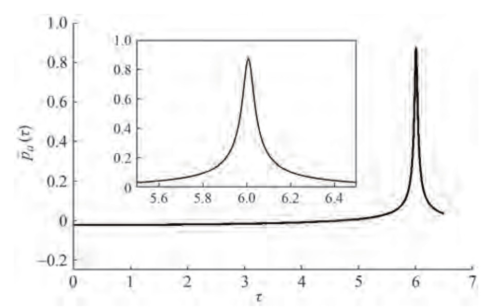 Figure 19 Dependence of nondimensional acoustic pressure on time during the collapse of gas-containing vapor bubbles moving along the contour of the rounded leading edge of elliptic hydrofoil at α/δ = 0.1
Table 3 presents the calculated data for the elliptical foil of relative thickness δ = 0.1.
Table 3 Spectral characteristics of impulses occurring at the collapse of gas-containing vapor bubbles on elliptic foil at an angle of attackα/δ τс $ \tilde{p}_a^{\max }$ σΔ Δτs 0.1 5.754 0.872 0.145 0.165 0.3 4.649 8.479 0.159 0.019 0.5 3.790 36.9 0.256 0.006 9 0.7 3.361 52.4 0.279 0.005 3 1.3 2.911 85.14 0.297 0.000 35 Sudden pressure increase 0.914 6 462.5 0.8 0.003 46  Figure 20 Acoustic impulse spectra at the collapse of gas-containing bubbles near the rounded leading edge of the elliptic foil for different angles of attack and relative thicknesses δ = 0.1
6 Conclusions
Some issues of dynamics and acoustics of a gas-containing vapor bubble moving in a variable pressure field are considered in this study. The analysis is by using analytical and numerical methods.
First, this paper reviews some classical results, which are most relevant to the compression process of a bubble suddenly entering an increased pressure zone. The dynamics of a bubble moving along the contour of the rounded leading edge of a thin and slightly curved hydrofoil at an angle of attack is then investigated. In the latter case, the local flow field is analytically described through the application of the MAE method. Therefore, the local distribution of pressure coefficient, its minimum magnitude, abscissas of critical points, and the point of minimal pressure have been obtained in closed form. The bubble originating at some point of the flow is viewed as a material point moving along a selected streamline in a corresponding variable pressure field, and its dynamics are examined using the Rayleigh-Plesset equation up to the moment of collapse. The MAE approach provides a direct way to investigate the influence of the foil angle of attack, thickness, and camber on bubble dynamics.
The results also include time dependencies of acoustic pressure induced by the contracting bubble up to its collapse, as well as some spectral characteristics. Most of the data are given in nondimensional format considering the similarity theory, easily enabling derivation of dimensional results for practical cases.
The present analysis has been performed for a 2D steadystate flow but can also be extended to 3D flows around wings and screw propellers. In the latter case, the outer expansion of the solution corresponds to a linear lifting surface theory. The local inner flow remains quasi-2D in the planes normal to the platform contour of the leading edge of the wing (or screw propeller blade). Typical contraction periods of the bubble, ending up with its collapse, are remarkably smaller compared with typical periods of almost any variation in the flow. Thus, the approach advocated in this paper can be applied to unsteady motions of the foil.
As noted by reviewers, an important role in the final stage of the bubble collapse can be played by thermal effects as the pressures and temperatures become remarkably high. Heat transfer can have notable influences on the bubble boundary motion. Nonequilibrium condensation effects can result in additional cushioning of the collapse. The Rayleigh-Plesset equation is coupled with the nonlinear energy equation to model these challenging phenomena.
-
Figure 1 Dynamics of vapor bubbles in the absence (solid line) and presence of the gas (dotted line)
Figure 2 Undamped oscillations of the bubble in the presence of gas (thick solid line: δg = 0 indicates the absence of gas, the solid line indicates δg = 0.01, and the dotted line indicates δg = 0.001)
Figure 3 Damped oscillations of gas-containing bubbles considering the capillarity and viscosity of the fluid (δg = 0.001, R0=10−5 m)
Figure 4 Influence of viscosity and capillarity on bubble dynamics under compression with no gas inside (dotted line) (the solid line corresponds to the compression curve for the bubble with no influence of viscosity and capillarity)
Figure 5 Division of the flow field around a foil (MAE)
Figure 6 Typical patterns of streamlines
Figure 7 Typical pattern of the local flow around the parabolic leading edge containing stagnation line (in stretched coordinates X and Y)
Figure 8 Distribution of pressure coefficient along the leading edge of the foil versus stretched abscissa X (ellipse, α = δ = 0.1)
Figure 9 Distribution of pressure coefficient along the leading edge of the foil versus stretched abscissa X (ellipse α =0.13, δ = 0.1)
Figure 10 Dependence of pressure coefficient on the stretched arc coordinate, measured from the critical point (ellipse, δ = 0.1)
Figure 11 Distribution of pressure coefficient along the leading edge of the elliptical; NACA66 m and Zhukovsky foil versus stretched abscissa X (δ = 0.1, α = 0.13)
Figure 12 Typical dependences of normalized radii of vapor bubbles on the nondimensional time for different magnitudes of the angle of attack and elliptical foil, δ = 0.1, R0 /rle = 0.2
Figure 13 Dependences of nondimensional time at which the bubble collapses on the ratio of the angle of attack (in radians) to the relative thickness of the foil for (κ = − pmin; δ = 0.1; R0 /rle = 0.2)
Figure 14 Bubble dynamics at κ < −pmin, κ = 3, δ = 0.1, α = 0.1, pmin = − 4.21, R0/rle = 0.2
Figure 15 Bubble dynamics at κ < −pmin, κ = 0.96, δ = 0.1, α = 0.07, pmin=−2.17, R0/rle = 0.2
Figure 16 Dependences of normalized radii of vapor bubbles on nondimensional time for different foils, α = 0.13, δ = 0.1, R0 /rle = 0.2
Figure 17 Nondimensional acoustic pressure versus nondimensional time (during the period of compression and near the moment of the bubble collapse)
Figure 18 Spectrum of acoustic pressure impulse during the collapse of gas-containing bubbles for the case of instantaneous pressure increase
Figure 19 Dependence of nondimensional acoustic pressure on time during the collapse of gas-containing vapor bubbles moving along the contour of the rounded leading edge of elliptic hydrofoil at α/δ = 0.1
Figure 20 Acoustic impulse spectra at the collapse of gas-containing bubbles near the rounded leading edge of the elliptic foil for different angles of attack and relative thicknesses δ = 0.1
Table 1 Quantities of ηmin and τc versus δg
δg ηmin τc 0 0 0.914 680 9 0.001 0.002 991 0.915 601 0.005 0.014 78 0.919 373 0.01 0.029 12 0.924 271 0.015 0.043 06 0.929 337 Table 2 Values uδ, uc and rle for different foil families
Foil type uδ uc rle Ellipse 1 0 1 NACA 66012 0.817 0 0.874 Gö (Walchner foil) 0.919 0.246 0.964 NACA4412 2 0.296 1.026 NACA66 m (a = 0.8) 0.75 0.208 0.848 Zhukovsky foil 2.288 0 2.35 Table 3 Spectral characteristics of impulses occurring at the collapse of gas-containing vapor bubbles on elliptic foil at an angle of attack
α/δ τс $ \tilde{p}_a^{\max }$ σΔ Δτs 0.1 5.754 0.872 0.145 0.165 0.3 4.649 8.479 0.159 0.019 0.5 3.790 36.9 0.256 0.006 9 0.7 3.361 52.4 0.279 0.005 3 1.3 2.911 85.14 0.297 0.000 35 Sudden pressure increase 0.914 6 462.5 0.8 0.003 46 -
Abbot IH, Von Doenhoff AE (1959) Theory of wing sections, including a summary of airfoil data. Dover Publications, Inc., New York Ahn JW, Park Ⅱ R, Park YH, Kim JI, Seol HS, Kim KS (2019) Influence of thru holes near leading edge of a model propeller on cavitation behavior. Journal of the Society of Naval Architects of Korea 56(3): 281-289. DOI: 10.3744/SNAK.2019.56.3.281 Benjamin TB, Ellis AT (1966) The collapse of cavitation bubbles and the pressures thereby produced against solid boundaries. Philosophical Transactions of the Royal Society B Biological Sciences, 260(1110): 221-240. DOI: 10.1098/rsta.1966.0046 Blake JR, Gibson DC (1987) Cavitation bubbles near boundaries. Ann. Rev. Fluid Mech. 19: 99-123 https://doi.org/10.1146/annurev.fl.19.010187.000531 Brennen CE (1995) Cavitation and bubble dynamics. Oxford University Press, New York-Oxford Briancon-Marjollet L, Franc JP, Michel JM (1988) Prediction of cavitation as a function of water nuclei content and hydrodynamic conditions (Case of the flow around a two-dimensional hydrofoil) Ceccio SL, Brennen SE (1991) Observations of the dynamics and acoustics of travelling bubble cavitation. Journal of Fluid Mechanics 233: 633-660 https://doi.org/10.1017/S0022112091000630 Chahine GL (1976) Asymptotic study of the behavior of a cavitation bubble in a variable pressure field. Journal de Mecanique 15(2): 286-306 Chahine GL (2009) Numerical simulation of bubble flow interactions. Journal of Hydrodynamics 21(3): 316-332. DOI: 10.1016/S1001-6058(08)60152-3 Egashira R (2016) Effects of the translational motion of a vapor bubble on its expansion or contraction in cavitation inception. Proceedings of the Fluid Engineering Conference, 0723. DOI: 10.1299/jsmefed.2016.0723 Franc JP (2007) The Raleigh-Plesset equation: a simple and powerful tool to understand various aspects of cavitation. Fluid Dynamics of Cavitation and Cavitating Turbopumps, CISM Courses and Lectures, 496, Springer, pp1-41, 978321176682. DOI: 10.1007/978-3-211-76669-9_1, hal-00265882 Franc JP, Michel JM (2004) Fundamentals of cavitation. In: Fluid Mechanics and its Applications Series, Vol. 76, Kluwer Academic Publishers Fuster D, Hauk G, Dopazo C (2009) Parametric analysis for a single collapsing bubble. Flow Turbulence and Combustion 82: 25-46. DOI: 10.1007/s10494-008-9169-8 Hsiao CN, Ma J, Chahine GL (2016) Numerical studies of bubble cloud dynamics near a rigid wall. Proceedings 31st Symposium on Naval Hydrodynamics, Monterey, USA Iben U, Makhnov A, Schmidt A (2018) Numerical study of a vapor bubble collapse near a solid wall. Journal of Physics Conference Series 1135: 012096. DOI: 10.1088/1742-6596/1135/1/012096 Lauterborn W, Ohl CD (1997) The peculiar dynamics of cavitation bubbles. Applied Scientific Research 58: 63-76. DOI: 10.1023/A:1000759029871 Levkovskiy YL (1968) Pressure field caused by the collapse of the cavitation cavity. Acoustical Journal 14(4): 239-243. (in Russian) Levkovskiy YL (1978) Structure of cavitating flows. Sudostroenie Publishers, Leningrad. (in Russian) Lindau O, Lauterborn W (2000) Laser-produced cavitation-studied with 100million frames per second. AIP Conference Proceedings 524(1): 385. https://doi.org/10/1063/1.1309247 Miniovich IA, Pernik AD, Petrovskiy VS (1972) Hydrodynamic sources of noise. Sudostroenie Publishers, Leningrad. (in Russian) Mishkevich VG, Rozhdestvensky KV (1978) Calculation of the flow past a thin hydrofoil on the basis of the method of matched expansions and its application for design of blade sections of screw propellers sections. Probl. S Shipbuild. Ser. Ship Des. 9: 96-106 Nigmatulin RI (1987) Dynamics of multiphase media. Part 1 (464 p.) and Part 2 (360 p.), Nauka Publishers, Moscow Plesset MS (1949) The dynamics of cavitation bubbles. J. Appl. Mech. 16(3): 277-282. https://doi.org/10.1115/1.4009975 Plesset MS (1996) Shockwaves from cavity collapse. Philosophical Transactions of the Royal Society B Biological Sciences 260(1110): 241-244 DOI: 10.1098/rsta.1966.0047 Plesset MS, Chapman RB (1971) Collapse of initially spherical vapor cavity in the neighborhood of solid boundary. J. Fluid Mech. 47(2): 283-290. DOI: 10.1017/S0022112071001058 Prosperetti A (2017) Vapor bubbles. Annual Review of Fluid Mechanics 49: 221-248 https://doi.org/10.1146/annurev-fluid-010816-060221 Rayleigh L (1917) On the pressure developed in a liquid during the collapse of a spherical cavity. Phil. Mag. 34 (200): 94-98. https://doi.org/10.1080/14786440808635681 Rusak Z (1994) Subsonic flow around the leading edge of a thin aerofoil with a parabolic nose. Eur. J. Appl. Math. 5: 283-311 https://doi.org/10.1017/S0956792500001479 Rusak Z, Morris WJ, Peles Y (2007) Prediction of leading-edge sheet cavitation inception on hydrofoils at low to moderate Reynolds number flows. Journal of Fluids Engineering 129(12): 1540-1546. DOI: 10.1115/1.2801350 Rozhdestvensky KV (1979) Method of matched asymptotic expansions in wing hydrodynamics. Sudostroenie Publishers, Leningrad. (in Russian) Rozhdestvensky KV, Mishkevich VG (1983) Calculation of unsteady flow past a thin foil on the basis of the matched asymptotic expansions method. Journal "Issues of shipbuilding", series "Ship design", 37: 60-73. (in Russian) Rozhdestvensky KV (2019) Study of unsteady flow near a rounded leading edge of a wing foil. J. of Marine Intellectual Technologies 1(43): 39-45. (in Russian) Trummler T, Schmidt SJ, Adams N (2021a) Numerical investigation of non-condensable gas effect on vapor bubble collapse. Physics of Fluids 33(9): 096107. DOI: 10.1063/5.0062399 Trummler T, Schmidt SJ, Adams N (2021b) Effect of stand-off distance and spatial resolution on the pressure impact of near-wall vapor bubble collapses. International Journal of Multiphase Flow 141(1): 103618. DOI: 0.1016/j.ijmultiphaseflow.2021.103618 Van-Dyke MD (1955) Second-order subsonic airfoil-section theory and its practical application. NACA Technical Note 3390, Ames Aeronautical Laboratory, Moffett Field, California, Washington Van-Dyke MD (1975) Perturbation methods in fluid mechanics. The Parabolic Press, Stanford Van Rijsbergen M, Lidtke AK (2020) Sheet cavitation inception mechanism on a NACA 0015 hydrofoil. Proceedings of the 33rd Symposium on Naval Hydrodynamics, Osaka Wang XY, Zhou SH, Shan ZM, Yin MG (2021) Investigation of cavitation bubble dynamics considering pressure fluctuation induced by slap forces. Mathematics 9(17): 2064. https://doi.org/10.3390/math9172064
| Citation: |
Kirill V. Rozhdestvensky (2022). Dynamics of Vapor Bubble in a Variable Pressure Field. Journal of Marine Science and Application, 21(3): 83-98. https://doi.org/10.1007/s11804-022-00289-4

|
